METHODS FOR ESTIMATION OF COUNTER MEASURES
TO IMPROVE
OSCILLATORY STABILITY IN POWER SYSTEMS
Simon P. Teeuwsen István Erlich Mohamed A. El-Sharkawi
University of Duisburg-Essen University of Duisburg-Essen University of Washington, Seattle
Abstract – This paper deals with computation of counter measures in case of insufficient damping of inter-area oscillations in large power systems. Inter-inter-area oscilla-tions have been observed many times in recent years. However, once a critical situation is identified, the opera-tor has to take counter measures, which ensure that the system moves back to a stable operating point. This study proposes a new method composed of Neural Networks and nonlinear optimization to estimate the best counter meas-ures. Thereby an optimization algorithm maximizes the predicted system damping by adjusting selected control variables in the power system. A Neural Network assesses the expected damping within the optimization loop. A second Neural Network is used to ensure feasible power flow conditions. The optimization results in a new power flow feature vector, which corresponds to a situation with higher damping than the current one. The result provides the Transmission System Operator important information about stability-improving actions he can run.
Keywords: Oscillatory Stability, Large Power Sys-tems, Optimization, Counter Measures, Damping Im-provement
1 INTRODUCTION
Inter-area oscillations in large-scale power systems are becoming more common especially for the Euro-pean Interconnected Power System UCTE/CENTREL. The system has grown very fast in a short period of time due to the recent east expansion. This extensive inter-connection alters the stability region of the network, and the system experiences inter-area oscillations associated with the swinging of many machines in one part of the system against machines in other parts. Moreover, for certain power flow conditions, the system damping changes widely [1], [2]. The deregulation of electricity markets in Europe aggravated the situation once more due to the increasing number of long distance power transmissions. Moreover, the network is becoming more stressed also by the transmission of wind power.
In fact, the European Power System is designed rather as a backup system to maintain power supply in case of power plant outages. The system is operated by several independent transmission utilities, joint by a large meshed high voltage grid. Because of the increas-ing long distance transmissions, the system steers closer to the stability limits. Thus, the operators need computa-tional real time tools for controlling system stability. Of main interest in the European Power System is hereby
the Oscillatory Stability Assessment (OSA). The use of on-line tools is even more complicated because Trans-mission System Operators (TSO) exchange only re-stricted information. Each TSO controls a particular part of the power system, but the exchange of data between different parts is limited to a small number because of the high competition between the utilities.
However, the classical small-signal stability compu-tation requires the entire system model and is time con-suming for large power systems [3]. Therefore, Compu-tational Intelligence (CI) methods for a fast on-line OSA based only on a small set of data became of high interest. Some CI methods were proposed recently [4] – [6]. These studies discuss the issues of oscillatory sta-bility in large interconnected power systems and solu-tions for on-line stability assessment using CI tech-niques. These techniques allow fast and accurate as-sessment of the current system state and provide there-fore helpful information for the TSO who runs the power system. In case of a critical situation, the TSO also would like to know how to prevent the system from collapse and which action will lead to a better damped power system. This information cannot be provided by the presented OSA method since it is designed for sta-bility assessment only.
The research area of counter measures deals with the problem, which operator action will have a stability improving impact on the power system. Of course, the system operator is trained to manage critical situations, but with the increasing complexity of the power sys-tems, especially in Europe, operator’s decision requires more and more computational tools. For this reason, this study suggests a CI based method, which allows the operator taking the most effective counter measures for steering the system to a more stable state.
2 16-MACHINE DYNAMIC TEST SYSTEM
winter and in summer, and change of the networks’ topology when transmission lines are switched.
Figure 1: One-Line Diagram of the PST 16-Machine Dy-namic Test System
To generate learning samples for CI methods, vari-ous power flow scenarios under the 5 operating condi-tions are considered. These scenarios are generated by real power exchange between 2 areas. The different power flow scenarios result in generating 5,360 patterns for learning.
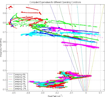
Figure 2: Computed Eigenvalues for the PST-Machine 16 Test System under different Power Flow Situations
The computed eigenvalues for all cases are shown in Figure 2. The slant lines in the figure are for constant damping at -2% to 4%. Different colors determine dif-ferent operating conditions like in summer and winter. As seen in the figure, most of the cases are for well-damped conditions, but in some cases the eigenvalues shift to the low damping region and can cause system instability.
3 CI BASED OSCILLATORY STABILITY ASSESSMENT
3.1 Selection of Information used for OSA
Stability assessment methods require input informa-tion to make reliable predicinforma-tions. These inputs are state
information from the power system and they will be measured when implemented in a real power system. Large power systems include much information such as transmission line flows, generated powers and demands, voltages, and voltage angles. However, any effective CI method requires a small number of inputs, which are selected from the set of state information and can be processed easily. When used with too many inputs, CI methods will lead to long processing times and cannot be managed well [8]. According to the corresponding literature, we call these inputs “features”. However, the selected features must represent the entire system, since a loss of information in the reduced set results in loss of both performance and accuracy in the CI methods. Be-cause large interconnected power systems are highly nonlinear and complex, the exact relationships between all features and their impact on stability cannot be for-mulated by simple rules. For this reason, feature selec-tion based on engineering judgment or physical knowl-edge only is not recommended in large power systems. Rather, it should be implemented according to a mathe-matical procedure or algorithm. The selection technique applied in this study is based on physical pre-selection, followed by the Principal Component Analysis (PCA) and the k-Means cluster algorithm [9]. The final group of features is selected from the clusters constructed by k-means and used as input for the following CI methods. In this study, 50 features are selected for OSA. These features are listed in Table 1.
Feature Symbol Number
Sum Generation per Area P 2
Sum Generation per Area Q 3
Generator Power Output P 1
Generator Power Output Q 4
Transmitted Power on Line P 15 Transmitted Power on Line Q 8
Bus Voltage V 8
Voltage Angle ϕ 9
Table 1: 50 Selected Features for OSA
3.2 Neural Networks based OSA
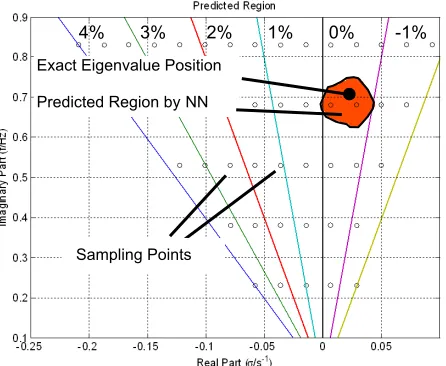
the positions of the eigenvalues. Thus, the distance between the eigenvalues and the samples is used to compute activation for the sampling points. The closer the distance between an eigenvalue and a sampling point, the higher the activation for this sampling point. The NN is trained with these activations. The advantage of this technique is the constant number of sampling points in the complex eigenvalue space, and therefore the NN structure is fixed once in the beginning and becomes independent of the number of dominant eigen-values. After NN training, the results are transformed from sampling point activations back into eigenvalue locations. The activations are used to setup a 3-dimensional activation surface by linear interpolation between all rows and columns of sampling points. The activation surface shows peaks at any position where dominant eigenvalues can be found. Then, a boundary surface of constant level is constructed, resulting from the minimum activation, which is necessary to detect an eigenvalue in the complex space. However, the intersec-tion of the activaintersec-tion surface and the boundary level leads to a 2-dimensional region in the complex space, which is called predicted region. These regions give information about locations of critical eigenvalues in the complex plain and therefore about the system damp-ing. An example for region prediction is shown in Fig-ure 3. The figFig-ure shows one dominant eigenvalue at about –0.5% damping computed for a given power flow scenario. The scenario is characterized by a high load winter condition with an additional real power transfer of 524 MW from area B in to power system to area C.
Figure 3: Computed Dominant Eigenvalue for a given Power Flow Scenario (Example 1) and Predicted Region Constructed by Eigenvalue Mapping
The lines in the figure are lines of constant damping and the sampling points resulting from the applied CI method are marked with circles. Then, the eigenvalue mapping is performed for this scenario and the resulting predicted region is plot into the figure, too. The pre-dicted region matches exactly the position of the domi-nant eigenvalue and demonstrates the accuracy of the CI method.
In the following, the NN is applied for eigenvalue region prediction. The NN is trained off-line with
sam-ple patterns. Then, it is used on-line to predict the power system minimum damping within milli-seconds. Because the NN is extremely fast in the prediction, it can be implemented in an algorithm to find counter measures as discussed in the next section.
4 COUNTER MEASURE ESTIMATION
4.1 Pre-Consideration
When the TSO runs the power system, there are a few items to be considered, which limit the possibilities of action. The TSO controls the power system, but his actions are limited to a few control variables only. Be-cause of contracts between utilities and customer, the TSO cannot change the generated real power at particu-lar power plants. He is also not able to change loads. However, by setting the transformer taps and/or reactive power infeed he can adjust the voltage level and control the power flow through transmission lines. Moreover, the generated reactive power can be influenced easily.
For this reason, at first, the set of features is de-scribed by 3 main characteristics, which are constant features, dependent features, and independent features. Constant features cannot be changed by the TSO like generated power and loads, respectively, and will be constant during the TSO’s actions. Dependent features also cannot be changed directly by the TSO, but they will change depending on the TSO’s action in the power system. Those features are most likely real and reactive power flows on transmission lines, voltage angles, and bus voltages. Finally, the independent features like transformer tap positions and generated reactive power can be changed by the TSO directly. The feature classi-fication is shown in Table 2.
4% 3% 2% 1% 0% -1%
Demand Voltage Angles
Table 2: Feature Classification according to their characteris-tics
Sampling Points
Control variables are those features in the power sys-tem, which are controlled by the TSO as described above. However, when the counter measure method is implemented, it is based on the feature vector selected for CI. But the feature vector contains only a few of those features, which are considered independent in the power system. Moreover, the feature vector does not include the transformer tap positions. For this reason, the control variables used in the counter measure com-putation are not only the independent features, but also the bus voltages. Bus voltages are controlled by trans-former tap positions and therefore they are indirectly independent.
4.2 Optimization Algorithm
using Neural Networks as cost and constraint function. The algorithm for cost function calculation performs classification and eigenvalue region prediction to de-termine the minimum-damping for the current system state. The minimum-damping coefficient is then maxi-mized by the optimization algorithm under the con-straint of a feasible power flow condition for the result-ing power flow.
In this paper we suggest to use NNs for both power flow adjustment and eigenvalue assessment as well. The application of NNs for OSA is discussed in [4] – [6] in detail. For the estimation of counter measures, we im-plement exactly the same NNs, which are used for OSA, too. The cost function of the optimization algo-rithm is calculated based on the eigenvalue regions predicted by these NNs.
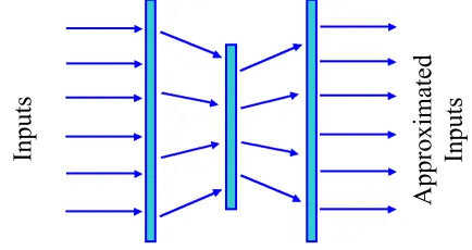
Figure 4: NN Auto Encoder for Input Feature Reproduction
A feasible power flow condition for the result is en-sured by the use of a NN auto encoder. The NN auto encoder is a well-known type of NN and discussed in detail in literature [10]. The application of NN auto encoder in power systems for power flow computation is introduced in [11]. This NN, shown in Figure 4, rep-licates the input vector at the output.
In other words, the NN is trained with various power flow conditions to obtain identical input and output. Therefore, the error between input and output vector will be low for any trained power flow condition. If the NN is trained properly, it is also able to identify new power flow conditions, which are not trained, by show-ing low errors between inputs and outputs. The squared sum of the differences between inputs and outputs is therefore a reliable measure for feasibility of the power flow corresponding to the presented feature vector. This error is used as constraint for the optimization to keep the possible power flow error within limits. If the error is low, the optimization assumes the power flow as feasible. If the error is high, the presented input vector does not belong to a feasible power flow condition, and therefore the optimization will continue.
During the entire optimization process, the features considered constant in Table 2 are kept constant. The control variables are the independent features and some bus voltages. They will be adjusted by the optimization algorithm in order to improve the predicted system damping. The dependent features are adapted to a feasi-ble power flow condition depending on the independent features by the NN auto encoder. The optimization block diagram is shown in Figure 5.
Figure 5: Nonlinear Sequential Quadratic Optimization Procedure for Damping Maximization
It is worth mentioning that the optimization results depend highly on the chosen optimization parameters. There exists not only one unique solution, but also many possible power flow conditions, which are stable and possible to reach from the initial starting condition.
Approximated
Inputs
The result of the optimization is a vector containing the new feature values for all dependent and independ-ent features. Once the power system power flow is adjusted to the new operating point, the system damping will increase to the optimized damping result.
Inputs
5 REALIZATION IN THE POWER SYSTEM
While the counter measure optimization is based on the feature vector including only a small set of control variables, the TSO has much more control variables in the real power system that can be changed. Since there is no need to use only those control variables, which are included in the counter measure computation, the TSO may control all control variables in the power system. This includes all transformer tap positions and the gen-erated reactive power at all generators, too.
For realization, this study uses a generalized OPF to reach the desired operating point in the power system. Commonly, OPFs for power flow computations are based on a target function to minimize the power system losses. However, in this case, a generalized OPF is developed for minimizing a target function defined as the difference between the desired features resulting from the counter measure computation and the actual power flow. When the new feature values are ap-proached in the system, it will result in damping im-provement. It is assumed that the generated real power is subjected to be constant because of the unbundling between power transmission utilities and power genera-tion utilities. Moreover, the power generagenera-tion depends on demand and power generation contracts and the TSO is not allowed to interact without emergency. When the new feature values are reached by the generalized OPF with good accuracy, it is expected that the system damping will be improved considerably. However, due to the restrictions changing the power flow, the effect regarding stability improvements will be usually less than expected.
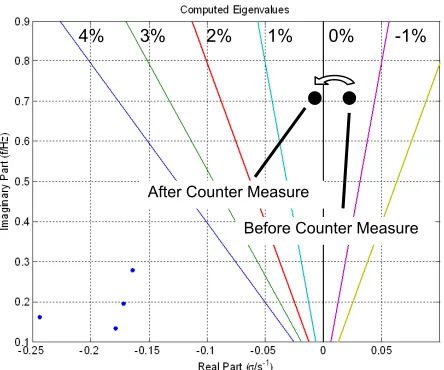
computed for this situation as described in the previous section. The CI input vector consists of 3 constant fea-tures, 39 dependent feafea-tures, and 8 control variables. The control variables are changed during the optimiza-tion whereas the 39 dependent features are adjusted by the NN auto encoder in order to keep the power flow feasible. The new eigenvalues for the scenario after the estimated counter measures are taken are shown in Figure 6. The initial location, before counter measures are taken, is plot to the figure as well. Compared to the original scenario, the eigenvalue has shifted slightly and thus the system damping has improved only marginally.
Figure 6: Computed Eigenvalues According to the Proposed Counter Measures (OPF Control Variables: Transformers and Generator Voltages) and Original Dominant Eigenvalue from Base Scenario (Example 1)
Because the improvement is not sufficient enough for any on-line tool, we decided to give the TSO more possibilities to act in the power system. Since the inter-area oscillations are mainly caused by the large power transit between area B and area C, we define the real power of two generators as independent features.
Figure 7: Computed Eigenvalues According to the Proposed Counter Measures (OPF Control Variables: Transformers, Generator Voltages, and Generated Real Power at two Gen-erators) and Original Dominant Eigenvalue from Base Sce-nario (Example 1)
One generator is located in area B and the other one is located in area C, and both are closed to the area-connecting tie line. In this case the real power genera-tion of those two generators can also be changed by the generalized OPF in order to reach the proposed targets. The results are shown in Figure 7.
The figure shows much more improvement in terms of system damping than Figure 6. This result leads to the conclusion, that the change of transformer tap posi-tions and reactive power is not sufficient in this particu-lar case to reach a well-damped system state. But when some selected real power sources are taken into account too, the transmitted power between distant areas is de-creased (real power transfer from area B to area C) and therefore the improvement can be enormous. A second example will demonstrate the impact of real power transits on the system stability. The basic scenario is a large power transit from area C to area A at the winter load condition. Both the computed eigenvalues for this scenario and the predicted region is shown in Figure 8.
4% 3% 2% 1% 0% -1%
After Counter Measure
Before Counter Measure
4% 3% 2% 1% 0% -1%
Computed Eigenvalue
Predicted Region
Figure 8: Computed Dominant Eigenvalue for a given Power Flow Scenario (Example 2) and Predicted Region Constructed by Eigenvalue Mapping
Counter measures are estimated to improve the sys-tem stability starting from the base situation described above and shown in Figure 8. When only transformer tap positions and generator voltages are variable in the optimization, the result is a slight decrease in system damping. The target features, estimated by the counter measure method, cannot be obtained by these variables. Therefore, the computed power flow situation is not the same as the power flow, which is proposed by the counter measure estimation. The system remains unsta-ble with a damping of –1%. This indicates the necessity of real power variation for damping improvement.
4% 3% 2% 1% 0% -1%
After Counter Measure
Figure 9: Computed Eigenvalues According to the Proposed Counter Measures (OPF Control Variables: Transformers, Generator Voltages, and Generated Real Power at two Gen-erators) and Original Dominant Eigenvalue from Base Sce-nario (Example 2)
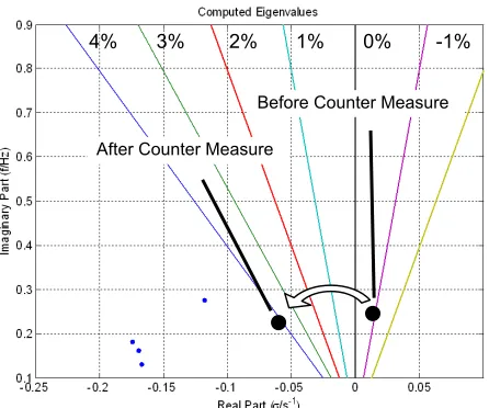
The counter measures are estimated once again for variable transformer tap positions, generator voltages, and generated real power at one selected generator, each in area A and area C. The OPF will run with the ex-tended degree of freedom changing control variables in the system. The result is a noticeable increase in system damping. The eigenvalues are shown in Figure 9 to-gether with the initial position of the dominant eigen-value, which has shifted towards the stable region with a damping of more than 4%. It is obvious, the critical situations in the investigated power system were caused by long distance real power transmissions. Therefore, counter measures are most effective when the generated real power at selected generators is taken into account, too.
6 CONCLUSION
This study shows a method how counter measures for an insufficient damped system can be estimated using only some selected power system information. The oscillatory stability is assessed first using CI techniques. Then, counter measures are estimated based on a nonlinear opti-mization algorithm where two NNs are engaged for eigen-value calculation and power flow feasibility. This method is fast and can be implemented as additional on-line tool for TSOs. The optimization result is a vector with new feature values providing the TSO information about a better-damped system state. For reaching the desired power flow, the TSO can take different control actions not necessarily considered in the previous feature calculation. This is e.g. changes in transformer tap positions. As a powerful tool, it is suggested to use a generalized OPF where the target function is defined as the difference be-tween the desired features resulting from the counter
measure computation and the actual power flow. This OPF can consider all control actions available to the TSO.
4% 3% 2% 1% 0% -1%
To achieve considerable damping improvement it may be necessary to change the real power flow be-tween areas swinging against each other. In the test system used in this study, control variables concerning mainly voltages and reactive power resulted in marginal improvements only. With allowing changing the real power generation in different areas, the generalized OPF was able to estimate a new power flow with no-ticeably better system damping.
Before Counter Measure
After Counter Measure
REFERENCES
[1] U. Bachmann, I. Erlich and E. Grebe, “Analysis of interarea oscillations in the European electric power system in synchronous parallel operation with the Central-European networks”, IEEE Pow-erTech, Budapest 1999
[2] H. Breulmann, E. Grebe, et al., “Analysis and Damping of Inter-Area Oscillations in the UCTE/CENTREL Power System”, CIGRE 38-113, Session 2000
[3] P. Kundur, Power System Stability and Control, McGraw-Hill, New York, 1994
[4] S.P. Teeuwsen, I. Erlich, M.A. El-Sharkawi, “Small-Signal Stability Assessment based on Ad-vanced Neural Network Methods”, IEEE PES General Meeting, Toronto, Canada, July, 2003 [5] S.P. Teeuwsen, I. Erlich, U. Bachmann,
“Small-Signal Stability Assessment of the European Power System based on Advanced Neural Net-work Method”, IFAC 2003, Seoul, Korea, Sep-tember, 2003
[6] S.P. Teeuwsen, Oscillatory Stability Assessment of Power Systems using Computational Intelli-gence, Aachen, Shaker, 2005
[7] S.P. Teeuwsen, I. Erlich, M.A. El-Sharkawi, “Neural Network based Classification Method for Small-Signal Stability Assessment”, IEEE Pow-erTech, Bologna, Italy, June, 2003
[8] M. Mendel, K.S. Fu, Adaptive, learning and pat-tern recognition systems: theory and applications, New York, Academic Press, 1972
[9] S.P. Teeuwsen, I. Erlich, M.A. El-Sharkawi, “Ad-vanced Method for Small-Signal Stability Assess-ment based on Neural Networks”, ISAP 2003, Lemnos, Greece, August/September 2003
[10] R.D. Reed and R.J. Marks, II, Neural Smithing, MIT Press, Cambridge, Mass.,1999