DOI 10.1007/s10640-009-9270-z
A Ricardian Analysis of the Distribution of Climate
Change Impacts on Agriculture across Agro-Ecological
Zones in Africa
S. Niggol Seo· Robert Mendelsohn · Ariel Dinar·
Rashid Hassan · Pradeep Kurukulasuriya
Received: 28 January 2009 / Accepted: 10 February 2009 / Published online: 3 March 2009 © Springer Science+Business Media B.V. 2009
Abstract This paper examines the distribution of climate change impacts across the six-teen Agro-Ecological Zones (AEZs) of Africa. We combine net revenue from livestock and
S. Niggol Seo is the Consultant to the World Bank. S. N. Seo (
B
)Basque Center for Climate Change, Bilbao, Spain e-mail: [email protected]
S. N. Seo
Research consultant to the World Bank; Research Associate, Yale University, Gran Via 35-2, Bilbao 48009, Spain
R. Mendelsohn
School of Forestry and Environmental Studies, Yale University, 195 Prospect Street, New Haven, CT 06511, USA
e-mail: [email protected] A. Dinar
Department of Environmental Sciences and Water Science and Policy Center, University of California, Riverside, CA, 92521, USA
e-mail: [email protected] A. Dinar
Development Economics Research Group, World Bank, Washington DC, 20433, USA R. Hassan
Department of Agricultural Economics, University of Pretoria, Pretoria, South Africa e-mail: [email protected]
R. Hassan
Center for Environmental Economics for Africa, University of Pretoria, Pretoria, South Africa P. Kurukulasuriya
Energy and Environment Group, Bureau of Development Policy, United Nations Development Programme, New York, USA
crops and regress total net revenue on a set of climate, soil, and socio-economic variables with and without country fixed effects. Although African crop net revenue is very sensitive to climate change, combined livestock and crop net revenue is more climate resilient. With the hot and dry CCC climate scenario, average damage estimates reach 27% by 2100, but with the mild and wet PCM scenario, African farmers will benefit. The analysis of AEZs implies that the effects of climate change will be quite different across Africa. For example, currently productive areas such as dry/moist savannah are more vulnerable to climate change while currently less productive agricultural zones such as humid forest or sub-humid AEZs become more productive in the future.
Keywords Climate change·Economic impacts·Agriculture·Africa·AEZ
1 Introduction
The most recent report of the Intergovernmental Panel on Climate Change provides strong
evidence of a warming world (Intergovernmental Panel on Climate Change (IPCC) 2007a).
Although there are many calls for international action, reducing greenhouse gases is costly. The international community needs to carefully weigh the costs and benefits of any program
of action (Nordhaus 2007). One of the major concerns about climate change is food security,
especially for people living in the low latitudes.
Previous global climate studies have predicted that climate change would have serious
impacts on agriculture in developing countries (Pearce et al. 1996;Tol 2002;Mendelsohn et
al. 2006). Early empirical studies using crop simulation models suggested that agriculture in
developing countries was highly vulnerable to warming (Rosenzweig and Parry 1994;Reilly
et al. 1996). Subsequent economic research using Ricardian models (Mendelsohn et al. 1994)
also suggests that developing country crops are vulnerable (Kurukulasuriya et al. 2006;Seo
and Mendelsohn 2008a).
These earlier studies provide useful measures of the impacts at a continental or national scale. However, there remains a question of how best to measure the impacts across the landscape. This study takes advantage of Agro-Ecological Zones (AEZs) to predict how impacts will be dispersed across the African landscape. The differential effects of climate change on farms in various agro-ecological zones have not yet been quantified. Specifically, we examine how climate change might affect farm net revenue in different AEZs. Not only does this research provide insights into how climate affects farmers facing different condi-tions, but it will also help extrapolate climate change results from the existing sample to the continent from which they are drawn.
This study combines the AEZs data with the farm economic data from a recently
com-pleted GEF/World Bank study of African agriculture (Dinar et al. 2008). The AEZs data are
compiled by the Food and Agriculture Organization of the United Nations using information
about climate, altitude, and soils (FAO 1978). The GEF/World Bank study measured crop
choice, livestock choice, yields, gross revenues, and net revenues of thousands of farmers
(households) in 11 African countries (Dinar et al. 2008). Both the countries and the farm
households were sampled across the various climates of Africa.
In addition to studying AEZs, this study makes another important contribution. Past stud-ies have focused on crops alone. The crop studstud-ies generally have concluded that the net
revenue from African crops will likely fall with warming (IPCC 2007b;Kurukulasuriya et
al. 2006;Kurukulasuriya and Mendelsohn 2008). However, the net revenue from African
This paper combines crop and livestock net revenue into total farm net revenue. The analysis simultaneously considers impacts on both crop and livestock.
In the next section, we briefly discuss the basic underlying theory of a Ricardian analy-sis. The third section describes the data. Empirical results are shown in the fourth section. We then use the estimated Ricardian model coefficients to predict climate change impacts by 2100 for two different climate scenarios. The paper concludes with a discussion of the results and policy implications.
2 Theory
Farmers in different AEZs employ different farm practices. Depending on the AEZ they are situated in, they will choose a specific farm type, irrigation, crop species, and livestock species that fit that AEZ. As some AEZs are better suited for agriculture while others are not, the average net revenues from these AEZs will differ.
In the Ricardian technique (Mendelsohn et al. 1994), adaptations are implicit and
endog-enous. The Ricardian technique assumes that each farmer maximizes net revenue subject to the exogenous conditions of the farm, which include climate. Net revenue is defined broadly to include own consumption as well as sold or traded products. The technique assumes each farmer chooses a mix of agricultural activities and inputs that provide the highest net reve-nue. The resulting net revenue across all farmers is therefore a function of just the exogenous variables:
π= f(P,C,W,S,H), (1)
whereπis net revenue per hectare,Pis a vector of input and output prices,Cis a vector of
climate variables and their squared terms,Wis available water for irrigation,Sis a vector
of soil characteristics, andHis a vector of household characteristics. The Ricardian model
estimates Eq.1econometrically by specifying a quadratic function of climate variables along
with other control variables. By grouping the various variables, the reduced form equation for net revenue becomes
π=Cβ+Sγ +Wϕ+Hλ+Pα+u (2)
whereu is an error term which is identically and independently Normal distributed. The
remaining symbols are coefficients to be estimated. Because this analysis is applied across multiple countries, it is quite possible that there are variables at the national level such as agricultural policies, trade policies, property rights, and interest rates that are not taken into account in the analysis. We consequently also explore a country fixed effects model that controls for these missing variables with country dummies.
π=Cβ+Sγ +Wϕ+Hλ+Pα+Lη+u (3)
whereLis a set of country dummies.
We expect that the net revenue of farming varies by AEZs. Certainly, desert areas are less suitable for farming except near oases. Lowland semi-arid areas may also not be a good place
for crops (Kurukulasuriya et al. 2006). High land moist forests may not serve as a good place
for animal husbandry (Seo and Mendelsohn 2008b). These underlying productivity
differ-ences will lead to varying profits across climate, soil, and altitude and thus across AEZs. For example, we anticipate that the marginal climate effects for temperature and precipitation
iis calculated:
wherebT,bT2 are parameter estimates of the linear and the quadratic term ofT. Note that
the parameters are not a function of each AEZ. Climate change has a different effect on each AEZ because the marginal impacts depend on the climate of the AEZ.
In order to measure the welfare value (W) of a change from one climate (CA) to another
climate (CB), we subtract the net revenue before the change from the net revenue after the
change for each farm household. The welfare change is the difference between the two cli-mates. If the value is negative (positive), profits declined (increased), then the climate change has caused damage (benefit):
W =π(CB)−π(CA) (5)
Because the Ricardian function is estimated across space at one moment of time, the level of prices as a function of aggregate output is constant. The model cannot capture how prices would change if global quantities of output changed. With international trade, this bias is not
expected to be large (Mendelsohn and Nordhaus 1996). However, if price changes were to
occur, they would offset changes in quantity, leading to a smaller change in net revenues. The omission of prices in the Ricardian method may lead the method to overestimate the actual damages. Note also that the welfare measure being considered above is a comparative equilibrium analysis. The Ricardian method is not intended to be a dynamic measurement of transition costs.
3 Description of Data
The FAO has developed a typology of AEZs as a mechanism to classify the growing potential
of land (FAO 1978). The AEZs are defined using the length of the growing season. The
grow-ing season, in turn, is defined as the period where precipitation and stored soil moisture is greater than half of the evapotranspiration. The longer the growing season, the more crops
can be planted (or in multiple seasons) and the higher are the yields (Fischer and van
Velthu-izen 1996;Voortman et al. 1999). FAO has classified land throughout Africa using this AEZ concept. Our study will use these FAO defined AEZ classifications.
The economic data for this study was collected by national teams (Dinar et al. 2008). The
data was collected for each plot within a household and household level data was constructed from the plot level data. In each country, districts were chosen to get a wide representation of farms across climate conditions in that country. The districts were not representative of the distribution of farms in each country as there are more farms in more productive locations. In each chosen district, a survey was conducted of randomly selected farms. The sampling was clustered in villages to reduce sampling cost. A total of 9,597 surveys were admin-istered across the 11 countries in the study. However, the data from Zimbabwe had to be dropped because of difficulties to accurately conduct the sampling and interviewing due to political turmoil during the data collection period. Further cleaning brought the number of observations down to 8,509. The number of surveys varied from country to country.
We rely on satellites for temperature data and ground stations for precipitation (Mendelsohn et al. 2007). The temperature data come from polar orbiting satellites
oper-ated by the US Department of Defense (Basist et al. 1998). The precipitation data come from
dataset, created by the National Oceanic and Atmospheric Association’s Climate Prediction Center, has interpolated precipitation between ground stations.
We explore alternative measures of seasonal climate including a two season and a four season model. However, the two season model provides more reliable estimates (the four season model is presented in the Appendix). The two seasons include winter and summer. In the southern hemisphere, summer is defined as the average of November–January and winter is the average of May–July. These seasonal definitions provide the best fit. The seasons in the northern hemisphere were adjusted to the opposite months of the year.
Soil data was obtained from FAO (2003). The FAO data provides information about the major and minor soils in each location as well as slope and texture. Data concerning the hydrology was obtained from the results of an analysis of climate change impacts on
Afri-can hydrology (Strzepek and McCluskey 2006). Using a hydrological model for Africa, the
authors calculated flow for each district in the surveyed countries. Data on elevation at the
centroid of each district was obtained from the United States Geological Survey (USGS
2004). The USGS data is derived from a global digital elevation model with a horizontal grid
spacing of 30 arc seconds (approximately one kilometer).
4 Empirical Results
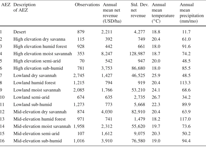
FAO has identified sixteen AEZs in Africa. Table1shows the classification of AEZs and
several descriptive statistics. The AEZs are classified by high, mid, and low elevation. Within each elevation, they are further broken down into five categories by the length of growing period: dry savannah, humid forest, moist savannah, semi-arid, and sub-humid. The other
remaining zone is desert. Farmers earn higher profits in high elevation moist savannah and sub humid zones and mid elevation dry savannah and sub humid zones. Farmers earn lower prof-its in high elevation dry savannah, humid forest, and semi arid zones, the lowland semi-arid zone, and in the desert zone.
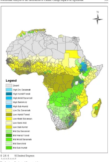
Figure1shows the distribution of the sixteen agro-ecological zones across the continent.
The Sahara desert occupies a vast land area in the north. There are also desert zones in the eastern edge and southern edge of the continent. Just beneath the Sahara in West Africa is a lowland semi-arid zone, followed by a lowland dry savannah, a lowland moist savannah, and a lowland sub-humid zone. The lowland humid forest then stretches from Cameroon across Central Africa. Eastern Africa is composed of some desert, lowland dry savannah, and some high elevation humid forest and dry savannah located around Mount Kilimanjaro and the highlands of Kenya. Southern Africa consists of lowland or mid elevation moist savannah, and lowland or mid elevation dry savannah.
Farms in different agro-ecological zones clearly face different conditions for farming. Hence, we expect that farms in favorable ecological zones for agriculture earn higher profits while farms in unfavorable zones earn much less per hectare. In order to examine the climate sensitivity of farms in each AEZ, we examine the variation of farm profits across different climate zones.
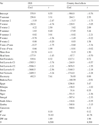
Since it is not clear whether Eqs.2or3is the best specification, we estimate both the OLS
and fixed effect model in Table2. The dependent variable is net revenue from both crops and
livestock divided by the hectares of cropland.1As many farmers in Africa consume their own
produce, we value own consumption at the market values of each product (Kurukulasuriya
et al. 2006;Seo and Mendelsohn 2008b,c). In addition, farmers use their own family labor at no pay. There is no observed wage rate for household labor and so it is not included as a cost. Net revenue thus includes returns to land and household labor. Household farms that rely mainly on their own labor may appear to have higher net revenue per hectare in comparison to commercial farms that rely on hired labor.
The estimated coefficients of the two regressions show that the response of net reve-nue to summer temperature is concave while the response to winter temperature is convex. Responses to summer and winter precipitation depend upon whether or not country fixed effects are included in the model. With the OLS model, precipitation is convex and with the country fixed effects model, precipitation is concave with respect to net revenue. Sum-mer climate interaction terms are generally negative and significant whereas winter climate interaction effects are positive but insignificant. Water flow and electricity coefficients are positive and strongly significant when country fixed effects are not included, but become insignificant when country fixed effects are introduced. Most of the significant soil coeffi-cients are negative. The country coefficoeffi-cients in the fixed effects model are positive for Egypt and Cameroon but negative for Niger, Burkina Faso, and Senegal. The OLS and fixed effects
models have similar adjusted R-squared,F-statistics, and Durbin Watson statistics, which
indicate that the empirical specifications are highly significant and not distorted by strong covariance among the observations.
Comparing the two models, it is evident that the country dummy variables are significant. They are clearly explaining some of the variation in net revenue. However, they are also capturing the differences in climate from country to country. The fixed effects model must estimate climate impacts relying solely on within country climate variation. It is not clear
Table 2 Ricardian regressions on net revenue (USD/ha)
Note: Dependent variable includes both crop and livestock net revenue
which of these two models is the best one to use for assessing policy interventions, so we include them both.
statistically significant. We also estimated a model that included all four seasons of the year
(see Appendix). In this case, the seasonal climate coefficients mostly become insignificant.2
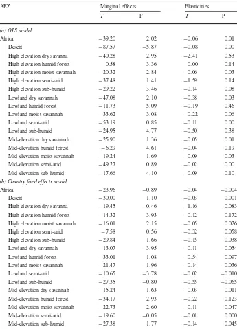
Because climate is introduced in a quadratic form, it is difficult to interpret the impact of
climate directly from the climate coefficients. Table3calculates the marginal change in net
revenue from a marginal change in temperature and precipitation for the models in Table2.
These marginal effects are calculated at the mean climate of each Agro-Ecological Zone. Higher temperatures are harmful. Net revenues fall as temperatures rise in every AEZ for both models. The largest negative impact is on high elevation dry savannah. The OLS model also predicts a large negative impact on high elevation semi-arid areas. Although both models predict temperature is harmful, they do not agree about the magnitude of the effect. The fixed effect model generally predicts smaller negative impacts from warming. However, this dif-ference between the models is not consistent. The fixed effect model predicts larger harmful impacts in more humid places whereas the OLS model predicts larger harmful impacts in dryer places.
Despite the fact that Africa is relatively dry, the two models do not agree that increased rainfall is beneficial. The OLS model implies more rain is generally beneficial, whereas the fixed effect model implies that rainfall is generally harmful. The OLS model predicts increased rainfall will be beneficial in all the AEZs except the desert. This odd result for the desert may have to do with the fact that desert agriculture depends strictly on irrigation. The fixed effect model predicts rainfall to be harmful for Africa but especially for high dry savannah and all lowland areas except humid forests. The fact that these results do not make sense is a serious deficiency of the fixed effect model.
5 Climate Predictions
The previous analysis suggests that temperature and precipitation currently have different effects on the net revenues in each AEZ. In this section, we explore the impacts future climate change scenarios may have on each AEZ. We use the estimated coefficients from the OLS and fixed effects models to predict long term impacts. However, we do not adjust earnings for other important factors that will change over the century such as capital investments, techno-logical change, and changes in prices. So it is important to remember that these predictions are just indications of the effect of climate change, not predictions of what may actually occur.
We use the country specific predictions of two climate models for 2100: CCC (Canadian
Climate Centre) (Boer et al. 2000) and PCM (Parallel Climate Model) (Washington 2000).
We use the A2 emission scenarios from the SRES report (IPCC 2000). These two scenarios
reflect the range of outcomes predicted in the most recent Intergovernmental Panel on
Cli-mate Change report (IPCC2007a). In each climate scenario, we add the predicted change in
temperature from the climate model to the baseline temperature for each season in each dis-trict. For precipitation, we multiply the predicted percentage change in precipitation from the
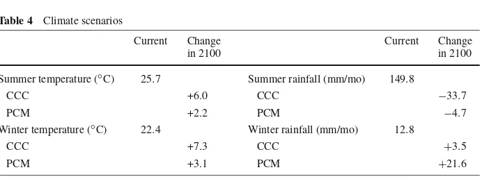
climate models by the baseline precipitation for each season in each district. Table4presents
the continental mean temperature and rainfall results. The PCM scenario is relatively mild
and wet and the CCC scenario is significantly hot and dry. The PCM predicts a 2◦C annual
increase and CCC a 6.5◦C annual increase in temperature. The PCM predicts a 10% increase
Table 3 Marginal effects and elasticities by AEZ
and, CCC a 15% decrease in annual mean rainfall. The predicted changes in each country varied slightly from these means depending on the climate scenario.
Table 4 Climate scenarios
Current Change in 2100
Current Change in 2100 Summer temperature (◦C) 25.7 Summer rainfall (mm/mo) 149.8
CCC +6.0 CCC −33.7
PCM +2.2 PCM −4.7
Winter temperature (◦C) 22.4 Winter rainfall (mm/mo) 12.8
CCC +7.3 CCC +3.5
PCM +3.1 PCM +21.6
same in the OLS and fixed effect models, the baseline values are different. The fixed effects model predicts higher baseline net revenues than the fixed effect model in desert, high ele-vation dry savannah and humid forest, mid eleele-vation humid forest, semi arid and sub-humid forest, and low elevation semi arid, sub-humid forest, and humid forest. In contrast, the OLS model predicts higher baseline net revenues in low elevation dry savannah, mid elevation dry savannah, and mid elevation moist savannah.
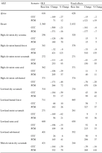
Future net revenues are calculated by multiplying the climate coefficients by future cli-mate. Climate change impacts are measured as the differences between net revenues in 2100
and net revenues in the baseline. The OLS results are shown in Table5. Both marginal
changes and percentage changes are presented for Africa for each AEZ. African farmers currently earn on average $630 per year for a hectare of land. The OLS model predicts that the PCM scenario leads to a 12% increase in net revenue and the CCC scenario leads to a 27% reduction in net revenue for Africa at large. The fixed effects model predicts similar but more positive results. The fixed effects model predicts that net revenue will rise by 19% with the PCM scenario and will fall by only 2% with the CCC scenario.
These relatively positive results for Africa contrast sharply with earlier more pessimistic
predictions for Africa (Kurukulasuriya et al. 2006;Kurukulasuriya and Mendelsohn 2008).
However, the earlier studies examined only crop net revenue. Studies on the livestock sector
suggested there would be offsetting gains (Seo and Mendelsohn 2008b,c). The analysis in
this paper, by combining both cropland and livestock net revenues, reveals a more moderate picture.
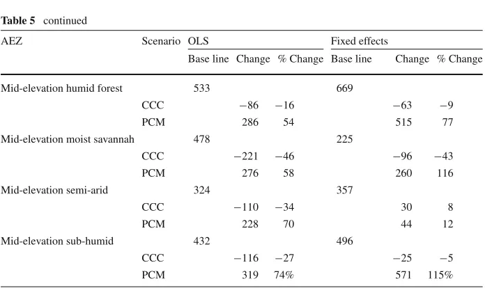
With the OLS model, the PCM scenario is beneficial in all AEZs but the desert. The CCC scenario is especially harmful in dry and moist savannah and high humid forests. However, the CCC scenario is expected to be slightly beneficial to lowland humid and sub-humid forest. With the fixed effects model, the only AEZ not predicted to gain under the PCM scenario is again the desert. The CCC scenario is expected to be harmful to high elevation moist savan-nah, humid forest, and sub-humid forest, and mid dry savansavan-nah, and humid forest. However, the CCC scenario is especially harmful to mid moist savannah.
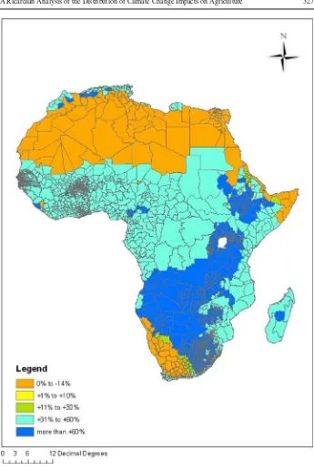
In Figs.2and3, we map the spatial distribution of the predicted impact from each of the
Table 5 Climate change impacts by AEZs and climate scenarios in 2100
AEZ Scenario OLS Fixed effects
Base line Change % Change Base line Change % Change
Table 5 continued
AEZ Scenario OLS Fixed effects
Base line Change % Change Base line Change % Change
Mid-elevation humid forest 533 669
This paper examines the role that climate plays in different AEZs in Africa. The paper relies on a cross-sectional analysis to assess the climate sensitivity of farms in each AEZ. The paper differs from previous studies in two important ways. It provides an analysis of total net revenue from both crops and livestock. Second, based on the AEZ classification, the analysis extrapolates impacts across the African landscape.
The paper compares Ricardian regressions with and without country dummies: OLS and fixed effect models. Both models reveal that climate variables are important determinants of farm net revenues in Africa. Summer and winter temperature and precipitation are all significant. A small increase in temperature would harm agricultural net revenues in Africa. The OLS model predicts that increased rainfall would increase net revenues whereas the fixed effect model predicts that increasing rainfall is harmful, but the rainfall effects vary by AEZs.
The estimated coefficients from both models were then used to predict climate change impacts for 2100 across a range of climate scenarios. The OLS model predicts that the PCM scenario leads to a 12% increase in net revenue, but the CCC scenario leads to a 27% reduc-tion in net revenue for Africa at large. The fixed effects model predicts that net revenue will rise by 19% with the PCM scenario, but will fall by 2% with the CCC scenario.
The results suggest that African agriculture is more resilient to climate change than what
earlier studies suggested (Rosenzweig and Parry 1994;Reilly et al. 1996;Kurukulasuriya et
al. 2006). We believe that this is because earlier studies examined only the impacts to crops whereas this study examines the impact on the combined net revenue of crops and livestock. There is evidence that some livestock are heat tolerant and that farmers will switch to these
species in hotter places and thus reduce their climate vulnerability (Seo and Mendelsohn
2008b,c).
Fig. 2 Percentage change of farm net revenue with CCC 2100 scenario
Fig. 3 Percentage change of farm net revenue with PCM 2100 scenario
Further, their economic and institutional ability to implement adaptation measures may also vary. Farmers facing similar climate situations may be affected differently, depending on other physical and economic/institutional conditions they face. Both physical and economic/insti-tutional conditions may affect the type of adaptation relevant for each location and the ability of the farmers residing in each location to adapt. Therefore, policy makers should consider tools that tailor assistance as needed. Policy makers should look carefully at impact assess-ments to identify the most attractive adaptation options. They should apply policies across the landscape using a ‘quilt’ rather than a ‘blanket’ approach. The proposed quilt policy approach will allow much more flexibility and will likely lead to much more effective and locally beneficial outcomes.
Several points can help in prioritizing, sequencing, and packaging interventions. First, even across the AEZs, policies that are designed in different countries should take into account the existing institutions and infrastructure in the country. While this advice may seem obvious, experience in replicating ‘best practices’ across countries and regions suggest that such considerations are not always taken into account.
The facts in Table1suggest that there is lot of variation between the AEZs in terms of the
population living in them and their net revenue. The analysis in the paper suggests that there is a large range of impacts across AEZs. Policy makers could sequence their interventions such that they address the most vulnerable AEZs first. This analysis does not lead to specific policy recommendations concerning what interventions are needed. However, it is clear that the indicated AEZ vulnerability is valid under many criteria: the population affected, the mean net revenue, and the total impacts.
The results presented in this paper, however, should be read with caution. First, the anal-ysis does not take into account the direct effects of carbon doubling which is believed to be beneficial to crop growth and may indirectly benefit livestock. Second, the study assumes agricultural prices, technology, inputs and capital remain the same for the coming century.
Third, it does not take into account transition costs involved in making adaptations (Kelly
et al. 2005). Finally, the analysis does not consider changes in policy that might take place that would either facilitate adaptation or make it more difficult.
Acknowledgements This work was supported by the World Bank. We want to thank David Maddison and Simon Dietz for their helpful comments on earlier drafts. The views are the authors alone.
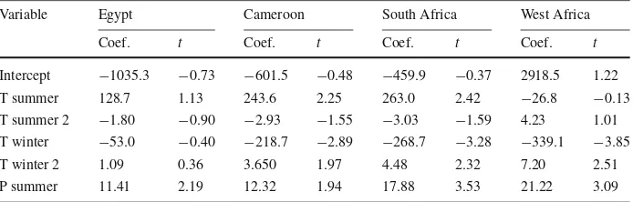
Appendix
See Tables6and7.
Table 6 Regression with country interaction terms
Variable Egypt Cameroon South Africa West Africa
Coef. t Coef. t Coef. t Coef. t
Intercept −1035.3 −0.73 −601.5 −0.48 −459.9 −0.37 2918.5 1.22
T summer 128.7 1.13 243.6 2.25 263.0 2.42 −26.8 −0.13
T summer 2 −1.80 −0.90 −2.93 −1.55 −3.03 −1.59 4.23 1.01 T winter −53.0 −0.40 −218.7 −2.89 −268.7 −3.28 −339.1 −3.85
T winter 2 1.09 0.36 3.650 1.97 4.48 2.32 7.20 2.51
Table 6 continued
Variable Egypt Cameroon South Africa West Africa
Coef. t Coef. t Coef. t Coef. t
P summer 2 −0.014 −1.81 −0.009 −0.66 −0.020 −2.56 −0.010 −1.22 P winter 3.97 0.58 −0.84 −0.12 −6.06 −0.82 −1.26 −0.17
P winter 2 0.021 1.10 0.023 1.08 0.027 1.41 0.032 1.34
T sum∗P sum −0.379 −2.00 −0.458 −2.3 −0.603 −3.28 −0.925 −3.03 T win∗P win −0.273 −0.77 −0.022 −0.06 0.241 0.61 −0.090 −0.19 T summer∗Dummy 2477.8 1.40 −21016.0 −4.13 8260.2 1.42 −70.8 −0.21 T summer 2∗Dummy −33.5 −1.00 444.1 4.14 −193.0 −1.51 −2.9 −0.49 T winter∗Dummy −3280.9 −4.38 6696.7 1.82 1051.1 0.54 310.3 0.55 T winter 2∗Dummy 124.6 2.38 −193.2 −2.04 −38.8 −0.36 −6.9 −0.58
Water flow 1238.1 0.74 1337.9 0.8 5430.5 0.95 880.6 0.52
Head farm −135.8 −0.32 −207.8 −0.47 −269.5 −0.62 −72.9 −0.16 Soil Ferralsols −3404.7 −1.36 −3773.9 −1.51 −5770.7 −1.60 −3838.9 −1.53 Soil Luvisols C1 −3168.8 −2.19 −3108.6 −2.15 2037.8 0.46 −3285.7 −2.26 Soil Luvisols C2 −1404.6 −1.84 −1675.0 −2.23 −2009.5 −1.69 −1796.5 −2.37
Soil Luvisols O 5.0 0.70 8.90 1.47 7.9 1.28 10.7 1.75
Soil Vertisols −93.3 −0.75 −77.7 −0.62 −78.8 −0.63 −90.2 −0.72
Electricity 80.2 1.04 67.9 0.87 78.1 1.01 73.0 0.94
Burkina Faso −16.7 −0.08 −268.7 −1.27 −199.8 −1.00 −151.4 −0.02
Egypt −18661.0 −0.76 1255.8 3.24 1195.6 2.96 958.8 2.04
Ethiopia −76.9 −0.57 −165.0 −1.18 −155.4 −1.15 −179.3 −1.24
Ghana 71.8 0.48 16.5 0.11 37.7 0.25
Niger −256.1 −1.06 −628.3 −2.56 −573.5 −2.43 Senegal −187.8 −0.82 −561.8 −2.44 −518.4 −2.33
South Africa 581.3 1.40 −111.5 −0.33 −90003.0 −1.50 −112.0 −0.28 Zambia −267.2 −1.44 −567.6 −3.15 −566.3 −3.20 −439.9 −2.00
Cameroon 1000.3 6.45 176917.0 3.67 959.5 6.17 1029.3 6.39
R2 0.12 0.12 0.12 0.12
F-stat 32.58 31.58 31.00 33.66
DW stat 1.95 1.94 1.93 1.93
N 8,509 8,509 8,509 8,509
References
Basist A, Peterson N, Peterson T, Williams C (1998) Using the Special Sensor Microwave Imager to mon-itor land surface temperature, wetness, and snow cover. J Appl Meteorol 37:888–911. doi:10.1175/ 1520-0450(1998)037<0888:UTSSMI>2.0.CO;2
Boer G, Flato G, Ramsden D (2000) A transient climate change simulation with greenhouse gas and aerosol forcing: projected climate for the 21st century. Clim Dyn 16:427–450. doi:10.1007/s003820050338
Dinar A, Hassan R, Mendelsohn R, Benhin J (eds) (2008) Climate change and agriculture in Africa: impact assessment and adaptation strategies. EarthScan, London, p189
FAO (1978) Report on Agro-Ecological Zones; vol 1: methodology and results for africa. Rome
Fischer G, van Velthuizen H (1996) Climate change and global agricultural potential: a case of Kenya. IIASA Working Paper WP-96-071
Food and Agriculture Organization (2003) The Digital Soil Map of the World (DSMW) CD-ROM. Italy, Rome. Available inhttp://www.fao.org/AG/agl/agll/dsmw.stm. Accessed March 2004
Intergovernmental Panel on Climate Change (IPCC) (2000) Special report on emissions scenarios. Cambridge University Press, Cambridge, UK
Intergovernmental Panel on Climate Change (IPCC) (2007a) The physical science basis. Fourth Assessment Report, Cambridge University Press, Cambridge, UK
Intergovernmental Panel on Climate Change (IPCC) (2007b) Impacts, adaptations, and vulnerability. Fourth Assessment Report, Cambridge University Press, Cambridge, UK
Kelly, DL, Kolstad CD, Mitchell G (2005) Adjustment costs from environmental change J Environ Econ Manag 50: 468–495
Kurukulasuriya P, Mendelsohn R (2008) A Ricardian analysis of the impact of climate change on African cropland. Afr J Agric Resour Econ 2:1–23
Kurukulasuriya P, Mendelsohn R, Hassan R, Benhin J, Diop M, Eid HM, Fosu KY, Gbetibouo G, Jain S, Mahamadou A, El-Marsafawy S, Ouda S, Ouedraogo M, Sène I, Maddision D, Seo N, Dinar A (2006) Will African agriculture survive climate change? World Bank Econ Rev 20:367–388. doi:10.1093/wber/ lhl004
Mendelsohn R, Nordhaus W (1996) The impact of global warming on agriculture: reply. Am Econ Rev 86:1312–1315
Mendelsohn R, Nordhaus W, Shaw D (1994) The impact of global warming on agriculture: a Ricardian anal-ysis. Am Econ Rev 84:753–771
Mendelsohn R, Dinar A, Williams L (2006) The distributional impact of climate change on rich and poor countries. Environ Dev Econ 11:1–20. doi:10.1017/S1355770X05002755
Mendelsohn R, Kurukulasuriya P, Basist A, Kogan F, Williams C (2007) Measuring climate change impacts with satellite versus weather station data. Clim Change 81:71–83. doi:10.1007/s10584-006-9139-x
Nordhaus W (2007) To tax or not to tax: alternative approaches to slow global warming. Rev Environ Econ Policy 1:22–44
Pearce D et al (1996) The social costs of climate change: greenhouse damage and benefits of control. In: Bruce J, Lee H, Haites E (eds) Climate change 1995: economic and social dimensions of climate change. Cambridge University Press, Cambridge, UK pp 179–224
Reilly J, Baethgen W, Chege F, van de Geijn S, Erda L, Iglesias A, Kenny G, Patterson D, Rogasik J, Rotter R, Rosenzweig C, Somboek W, Westbrook J (1996) Agriculture in a changing climate: impacts and adap-tations. In: Watson R, Zinyowera M, Moss R, Dokken D (eds) Climate change 1995: intergovernmental panel on climate change impacts, adaptations, and mitigation of climate change. Cambridge University Press, Cambridge, UK
Rosenzweig C, Parry M (1994) Potential impact of climate change on world food supply. Nature 367:133–138. doi:10.1038/367133a0
Seo SN, Mendelsohn R (2008a) A Ricardian analysis of the impact of climate change on South American farms. Chil J Agri Res 68:69–79
Seo SN, Mendelsohn R (2008b) Animal husbandry in Africa: climate change impacts and adaptations. Afr J Agric Resour Econ 2:65–82
Seo SN, Mendelsohn R (2008c) Measuring impacts and adaptations to climate change: a structural Ricardian model of African livestock management. Agric Econ 38:151–165
Strzepek K, McCluskey A (2006) District level hydroclimatic time series and scenario analyses to assess the impacts of climate change on regional water resources and agriculture in Africa. CEEPA Discussion Paper No. 13, Centre for Environmental Economics and Policy in Africa, University of Pretoria Tol R (2002) Estimates of the damage costs of climate change. Part 1: benchmark estimates. Environ Resour
USGS (United States Geological Survey) (2004) Global 30 arc second elevation data, USGS National Mapping Division, EROS Data Centre.http://edcdaac.usgs.gov/gtopo30/gtopo30.asp
Voortman R, Sonnedfeld B, Langeweld J, Fischer G, Van Veldhuizen H (1999) Climate change and global agricultural potential: a case of Nigeria. Centre for World Food Studies. Vrije Universiteit, Amsterdam Washington W et al (2000) Parallel climate model (PCM): control and transient scenarios. Clim Dyn 16:755–
774