Series editors
M.J. Carey S. CeriRajeev Rastogi
Editors
Data Stream Management
Minos Garofalakis School of Electrical and Computer Engineering Technical University of Crete Chania, Greece
Johannes Gehrke Microsoft Corporation Redmond, WA, USA
Rajeev Rastogi Amazon India Bangalore, India
ISSN 2197-9723 ISSN 2197-974X (electronic)
Data-Centric Systems and Applications
ISBN 978-3-540-28607-3 ISBN 978-3-540-28608-0 (eBook) DOI 10.1007/978-3-540-28608-0
Library of Congress Control Number: 2016946344
Springer Heidelberg New York Dordrecht London © Springer-Verlag Berlin Heidelberg 2016
The fourth chapter in part 4 is published with kind permission of © 2004 Association for Computing Machinery, Inc.. All rights reserved.
This work is subject to copyright. All rights are reserved by the Publisher, whether the whole or part of the material is concerned, specifically the rights of translation, reprinting, reuse of illustrations, recitation, broadcasting, reproduction on microfilms or in any other physical way, and transmission or information storage and retrieval, electronic adaptation, computer software, or by similar or dissimilar methodology now known or hereafter developed.
The use of general descriptive names, registered names, trademarks, service marks, etc. in this publication does not imply, even in the absence of a specific statement, that such names are exempt from the relevant protective laws and regulations and therefore free for general use.
The publisher, the authors and the editors are safe to assume that the advice and information in this book are believed to be true and accurate at the date of publication. Neither the publisher nor the authors or the editors give a warranty, express or implied, with respect to the material contained herein or for any errors or omissions that may have been made.
Printed on acid-free paper
Data Stream Management: A Brave New World . . . 1 Minos Garofalakis, Johannes Gehrke, and Rajeev Rastogi
Part I Foundations and Basic Stream Synopses
Data-Stream Sampling: Basic Techniques and Results . . . 13 Peter J. Haas
Quantiles and Equi-depth Histograms over Streams . . . 45 Michael B. Greenwald and Sanjeev Khanna
Join Sizes, Frequency Moments, and Applications . . . 87 Graham Cormode and Minos Garofalakis
Top-kFrequent Item Maintenance over Streams . . . 103 Moses Charikar
Distinct-Values Estimation over Data Streams . . . 121 Phillip B. Gibbons
The Sliding-Window Computation Model and Results . . . 149 Mayur Datar and Rajeev Motwani
Part II Mining Data Streams
Clustering Data Streams . . . 169 Sudipto Guha and Nina Mishra
Mining Decision Trees from Streams . . . 189 Geoff Hulten and Pedro Domingos
Frequent Itemset Mining over Data Streams . . . 209 Gurmeet Singh Manku
Temporal Dynamics of On-Line Information Streams . . . 221 Jon Kleinberg
Part III Advanced Topics
Sketch-Based Multi-Query Processing over Data Streams . . . 241 Alin Dobra, Minos Garofalakis, Johannes Gehrke, and Rajeev Rastogi
Approximate Histogram and Wavelet Summaries of Streaming Data . . 263 S. Muthukrishnan and Martin Strauss
Stable Distributions in Streaming Computations . . . 283 Graham Cormode and Piotr Indyk
Tracking Queries over Distributed Streams . . . 301 Minos Garofalakis
Part IV System Architectures and Languages
STREAM: The Stanford Data Stream Management System . . . 317 Arvind Arasu, Brian Babcock, Shivnath Babu, John Cieslewicz,
Mayur Datar, Keith Ito, Rajeev Motwani, Utkarsh Srivastava, and Jennifer Widom
The Aurora and Borealis Stream Processing Engines . . . 337 U˘gur Çetintemel, Daniel Abadi, Yanif Ahmad, Hari Balakrishnan,
Magdalena Balazinska, Mitch Cherniack, Jeong-Hyon Hwang, Samuel Madden, Anurag Maskey, Alexander Rasin, Esther Ryvkina, Mike Stonebraker, Nesime Tatbul, Ying Xing, and Stan Zdonik
Extending Relational Query Languages for Data Streams . . . 361 N. Laptev, B. Mozafari, H. Mousavi, H. Thakkar, H. Wang, K. Zeng,
and Carlo Zaniolo
Hancock: A Language for Analyzing Transactional Data Streams . . . 387 Corinna Cortes, Kathleen Fisher, Daryl Pregibon, Anne Rogers, and
Frederick Smith
Sensor Network Integration with Streaming Database Systems . . . 409 Daniel Abadi, Samuel Madden, and Wolfgang Lindner
Part V Applications
Stream Processing Techniques for Network Management . . . 431 Charles D. Cranor, Theodore Johnson, and Oliver Spatscheck
High-Performance XML Message Brokering . . . 451 Yanlei Diao and Michael J. Franklin
Adaptive, Automatic Stream Mining . . . 499 Spiros Papadimitriou, Anthony Brockwell, and Christos Faloutsos
Minos Garofalakis, Johannes Gehrke, and Rajeev Rastogi
1 Introduction
Traditional data-management systems software is built on the concept of persis-tent data setsthat are stored reliably in stable storage and queried/updated several times throughout their lifetime. For several emerging application domains, how-ever, data arrives and needs to be processed on a continuous (24×7) basis, without the benefit of several passes over a static, persistent data image. Suchcontinuous data streamsarise naturally, for example, in the network installations of large Tele-com and Internet service providers where detailed usage information (Call-Detail-Records (CDRs), SNMP/RMON packet-flow data, etc.) from different parts of the underlying network needs to be continuously collected and analyzed for interest-ing trends. Other applications that generate rapid, continuous and large volumes of stream data include transactions in retail chains, ATM and credit card operations in banks, financial tickers, Web server log records, etc. In most such applications, the data stream is actually accumulated and archived in a database-management system of a (perhaps, off-site) data warehouse, often making access to the archived data prohibitively expensive. Further, the ability to make decisions and infer interesting
M. Garofalakis (
B
)School of Electrical and Computer Engineering, Technical University of Crete, University Campus—Kounoupidiana, Chania 73100, Greece
e-mail:[email protected]
J. Gehrke
Microsoft Corporation, One Microsoft Way, Redmond, WA 98052-6399, USA e-mail:[email protected]
R. Rastogi
Amazon India, Brigade Gateway, Malleshwaram (W), Bangalore 560055, India e-mail:[email protected]
© Springer-Verlag Berlin Heidelberg 2016
M. Garofalakis et al. (eds.),Data Stream Management,
Data-Centric Systems and Applications, DOI10.1007/978-3-540-28608-0_1
Fig. 1 ISP network monitoring data streams
patternson-line(i.e., as the data stream arrives) is crucial for several mission-critical tasks that can have significant dollar value for a large corporation (e.g., telecom fraud detection). As a result, recent years have witnessed an increasing interest in designing data-processing algorithms that work over continuous data streams, i.e., algorithms that provide results to user queries while looking at the relevant data itemsonly once and in a fixed order(determined by the stream-arrival pattern).
Example 1(Application: ISP Network Monitoring) To effectively manage the op-eration of their IP-network services, large Internet Service Providers (ISPs), like AT&T and Sprint, continuously monitor the operation of their networking infras-tructure at dedicated Network Operations Centers (NOCs). This is truly a large-scale monitoring task that relies on continuously collecting streams of usage information from hundreds of routers, thousands of links and interfaces, and blisteringly-fast sets of events at different layers of the network infrastructure (ranging from fiber-cable utilizations to packet forwarding at routers, to VPNs and higher-level trans-port constructs). These data streams can be generated through a variety of network-monitoring tools (e.g., Cisco’s NetFlow [10] or AT&T’s GigaScope probe [5] for monitoring IP-packet flows), For instance, Fig.1depicts an example ISP monitoring setup, with an NOC tracking NetFlow measurement streams from four edge routers in the networkR1–R4. The figure also depicts a small fragment of the streaming
data tables retrieved from routersR1andR2containing simple summary
informa-tion for IP sessions. In real life, such streams are truly massive, comprising hundreds of attributes and billions of records—for instance, AT&T collects over one terabyte of NetFlow measurement data from its production network each day!
it is crucial to process and analyze these continuous network-measurement streams in real-time and a single pass over the data (as it is streaming into the NOC), while, of course, remaining within the resource (e.g., CPU and memory) constraints of the NOC. (Recall that these data streams are truly massive, and there may be hundreds or thousands of analysis queries to be executed over them.)
This volume focuses on thetheory and practice of data stream management, and the difficult, novel challenges this emerging domain introduces for data-management systems. The collection of chapters (contributed by authorities in the field) offers a comprehensive introduction to both the algorithmic/theoretical foun-dations of data streams and the streaming systems/applications built in different domains. In the remainder of this introductory chapter, we provide a brief summary of some basic data streaming concepts and models, and discuss the key elements of a generic stream query processing architecture. We then give a short overview of the contents of this volume.
2 Basic Stream Processing Models
When dealing with structured, tuple-based data streams (as in Example 1), the streaming data can essentially be seen as rendering massive relational table(s) through a continuous stream of updates(that, in general, can comprise both in-sertions and deletions). Thus, the processing operations users would want to per-form over continuous data streams naturally parallel those in conventional database, OLAP, and data-mining systems. Such operations include, for instance, relational selections, projections, and joins, GROUP-BY aggregates and multi-dimensional data analyses, and various pattern discovery and analysis techniques. For several of these data manipulations, the high-volume and continuous (potentially, unbounded) nature of real-life data streams introduces novel, difficult challenges which are not addressed in current data-management architectures. And, of course, such chal-lenges are further exacerbated by the typical user/application requirements for tinuous, near real-time results for stream operations. As a concrete example, con-sider some of example queries that a network administrator may want to support over the ISP monitoring architecture depicted in Fig.1.
• To analyze frequent traffic patterns and detect potential Denial-of-Service (DoS) attacks, an example analysis query could be: Q1:“What are the top-100 most fre-quent IP (source, destination) pairs observed at router R1 over the past week?”. This is an instance of atop-k (or, “heavy-hitters”)query—viewing theR1 as a (dynamic) relational table, it can be expressed using the standard SQL query language as follows:
Q1: SELECT ip_source, ip_dest, COUNT(*) AS frequency
FROM R1
• To correlate traffic patterns across different routers (e.g., for the purpose of dy-namic packet routing or traffic load balancing), example queries might include: Q2:“How many distinct IP (source, destination) pairs have been seen by both R1 and R2, but notR3?”, and Q3:“Count the number of session pairs in R1 and R2 where the source-IP in R1 is the same as the destination-IP in R2.”Q2 and Q3 are examples of (multi-table)set-expressionandjoin-aggregatequeries, respectively; again, they can both be expressed in standard SQL terms over theR1–R3 tables: Q2: SELECT COUNT(*) FROM
((SELECT DISTINCT ip_source, ip_dest FROM R1 INTERSECT
SELECT DISTINCT ip_source, ip_dest FROM R2 ) EXCEPT
SELECT DISTINCT ip_source, ip_dest FROM R3)
Q3: SELECT COUNT(*)
FROM R1, R2
WHERE R1.ip_source = R2.ip_dest
A data-stream processing engine turns the paradigm of conventional database systems on its head: Databases typically have to deal with a stream of queries over a static, bounded data set; instead, a stream processing engine has to effectively process a static set of queries over continuous streams of data. Such stream queries can be (i)continuous, implying the need for continuous, real-time monitoring of the query answer over the changing stream, or (ii)ad-hocquery processing requests interspersed with the updates to the stream. The high data rates of streaming data might outstrip processing resources (both CPU and memory) on a steady or intermit-tent (i.e., bursty) basis; in addition, coupled with the requirement for near real-time results, they typically render access to secondary (disk) storage completely infeasi-ble.
In the remainder of this section, we briefly outline some key data-stream man-agement concepts and discuss basic stream-processing models.
2.1 Data Streaming Models
An equivalent view of a relational data stream is that of a massive, dynamic, one-dimensional vector A[1. . . N]—this is essentially using standard techniques (e.g., row- or column-major). As a concrete example, Fig. 2 depicts the stream vector A for the problem of monitoring active IP network connections between source/destination IP addresses. The specific dynamic vector has 264entries captur-ing the up-to-date frequencies for specific (source, destination) pairs observed in IP connections that are currently active. The sizeN of the streamingAvector is de-fined as the product of the attribute domain size(s) which can easily grow very large, especially for multi-attribute relations.1The dynamic vectorAis rendered through
Fig. 2 Example dynamic vector modeling streaming network data
a continuous stream of updates, where thejth update has the general formk, c[j] and effectively modifies thekth entry ofAwith the operationA[k] ←A[k] +c[j]. We can define three generic data streaming models [9] based on the nature of these updates:
• Time-Series Model.In this model, thejth update isj,A[j]and updates arrive in increasing order ofj; in other words, we observe the entries of the streaming vector Aby increasing index. This naturally models time-seriesdata streams, such as the series of measurements from a temperature sensor or the volume of NASDAQ stock trades over time. Note that this model poses a severe limitation on the update stream, essentially prohibiting updates from changing past (lower-index) entries inA.
• Cash-Register Model.Here, the only restriction we impose on thejth update k, c[j]is thatc[j] ≥0; in other words, we only allow increments to the entries ofAbut, unlike the Time-Series model, multiple updates can increment a given entryA[j]over the stream. This is a natural model for streams where data is just inserted/accumulated over time, such as streams monitoring the total packets exchanged between two IP addresses or the collection of IP addresses accessing a web server. In the relational case, a Cash-Register stream naturally captures the case of anappend-onlyrelational table which is quite common in practice (e.g., the fact table in a data warehouse [1]).
• Turnstile Model.In this, most general, streaming model, no restriction is im-posed on thejth updatek, c[j], so thatc[j]can be either positive or negative; thus, we have a fully dynamic situation, where items can be continuously inserted and deleted from the stream. For instance, note that our example stream for moni-toring active IP network connections (Fig.2) is a Turnstile stream, as connections can be initiated or terminated between any pair of addresses at any point in the stream. (A technical constraint often imposed in this case is thatA[j] ≥0 always holds—this is referred to as thestrictTurnstile model [9].)
Turn-stile model (and, thus, are also applicable in the other two models). On the other hand, the weaker streaming models rely on assumptions that can be valid in certain application scenarios, and often allow for more efficient algorithmic solutions in cases where Turnstile solutions are inefficient and/or provably hard.
Our generic goal in designing data-stream processing algorithms is tocompute functions (or, queries) on the vectorAat different points during the lifetime of the stream (continuous or ad-hoc). For instance, it is not difficult to see that the exam-ple queries Q1–Q3 mentioned earlier in this section can be trivially computed over stream vectors similar to that depicted in Fig.2, assuming that the complete vec-tor(s) are available; similarly, other types of processing (e.g., data mining) can be easily carried out over the full frequency vector(s) using existing algorithms. This, however, is an unrealistic assumption in the data-streaming setting: The main chal-lenge in the streaming model of query computation is that the size of the stream vec-tor,N, is typically huge, making it impractical (or, even infeasible) to store or make multiple passes over the entire stream. The typical requirement for such stream pro-cessing algorithms is that they operate insmall spaceandsmall time, where “space” refers to the working space (or, state) maintained by the algorithm and “time” refers to both the processing time per update (e.g., to appropriately modify the state of the algorithm) and the query-processing time (to compute the current query answer). Furthermore, “small” is understood to mean a quantity significantly smaller than (N )(typically, poly-logarithmic inN).
2.2 Incorporating Recency: Time-Decayed and Windowed Streams
Streaming data naturally carries a temporal dimension and a notion of “time”. The conventional data streaming model discussed thus far (often referred to aslandmark streams) assumes that the streaming computation begins at a well defined starting pointt0(at which the streaming vector is initialized to all zeros), and at any time
t takes into account all streaming updates betweent0 andt. In many applications,
Fig. 3 General stream query processing architecture
3 Querying Data Streams: Synopses and Approximation
A generic query processing architecture for streaming data is depicted in Fig.3. In contrast to conventional database query processors, the assumption here is that a stream query-processing engine is allowed to see the data tuples in relationsonly once and in the fixed order of their arrivalas they stream in from their respective source(s). Backtracking over a stream and explicit access to past tuples is impossi-ble; furthermore, the order of tuples arrival for each streaming relation is arbitrary and duplicate tuples can occur anywhere over the duration of the stream. Further-more, in the most general turnstile model, the stream rendering each relation can comprise tuple deletions as well as insertions.
Consider a (possibly, complex) aggregate query Q over the input streams and letN denote an upper bound on the total size of the streams (i.e., the size of the complete stream vector(s)). Our data-stream processing engine is allowed a certain amount of memory, typically orders of magnitude smaller than the total size of its inputs. This memory is used to continuously maintain concisesynopses/summaries of the streaming data (Fig.3). The two key constraints imposed on such stream synopses are:
(1) Single Pass—the synopses are easily maintained, during a single pass over the streaming tuples in the (arbitrary) order of their arrival; and,
(2) Small Space/Time—the memory footprint as well as the time required to up-date and query the synopses is “small” (e.g., poly-logarithmic inN).
In addition, two highly desirable properties for stream synopses are:
(3) Delete-proof—the synopses can handle both insertions and deletions in the up-date stream (i.e., general turnstile streams); and,
At any point in time, the engine can process the maintained synopses in order to obtain an estimate of the query result (in a continuous or ad-hoc fashion). Given that the synopsis construction is an inherently lossy compression process, exclud-ing very simple queries, these estimates are necessarilyapproximate—ideally, with some guarantees on the approximation error. These guarantees can be either de-terministic(e.g., the estimate is always guaranteed to be withinǫrelative/absolute error of the accurate answer) orprobabilistic(e.g., estimate is withinǫerror of the accurate answer except for some small failure probabilityδ). The properties of such ǫ- or (ǫ, δ)-estimates are typically demonstrated through rigorous analyses using known algorithmic and mathematical tools (including, sampling theory [2,11], tail inequalities [7,8], and so on). Such analyses typically establish a formal tradeoff between the space and time requirements of the underlying synopses and estimation algorithms, and their corresponding approximation guarantees.
Several classes of stream synopses are studied in the chapters that follow, along with a number of different practical application scenarios. An important point to note here is that there really is no “universal” synopsis solution for data stream processing: to ensure good performance, synopses are typically purpose-built for the specific query task at hand. For instance, we will see different classes of stream synopses with different characteristics (e.g., random samples and AMS sketches) for supporting queries that rely onmultiset/bag semantics(i.e., the full frequency distribution), such as range/join aggregates, heavy-hitters, and frequency moments (e.g., example queries Q1 and Q3 above). On the other hand, stream queries that rely on set semantics, such as estimating the number of distinct values (i.e., set cardinality) in a stream or a set expression over a stream (e.g., query Q2 above), can be more effectively supported by other classes of synopses (e.g., FM sketches and distinct samples). A comprehensive overview of synopsis structures and algorithms for massive data sets can be found in the recent survey of Cormode et al. [4].
4 This Volume: An Overview
The collection of chapters in this volume (contributed by authorities in the field) offers a comprehensive introduction to both the algorithmic/theoretical foundations of data streams and the streaming systems/applications built in different domains. The authors have also taken special care to ensure that each chapter is, for the most part, self-contained, so that readers wishing to focus on specific streaming tech-niques and aspects of data-stream processing, or read about particular streaming systems/applications can move directly to the relevant chapter(s).
algorithms and synopses for more complex queries and analytics, and techniques for querying distributed streams. The chapters in Part IV focus on the system and lan-guage aspects of data stream processing through comprehensive surveys of existing system prototypes and language designs. Part V then presents some representative applications of streaming techniques in different domains, including network man-agement, financial analytics, time-series analysis, and publish/subscribe systems. Finally, we conclude this volume with an overview of current data streaming prod-ucts and novel application domains (e.g., cloud computing, big data analytics, and complex event processing), and discuss some future directions in the field.
References
1. S. Chaudhuri, U. Dayal, An overview of data warehousing and OLAP technology. ACM SIG-MOD Record26(1) (1997)
2. W.G. Cochran,Sampling Techniques, 3rd edn. (Wiley, New York, 1977)
3. E. Cohen, M.J. Strauss, Maintaining time-decaying stream aggregates. J. Algorithms59(1), 19–36 (2006)
4. G. Cormode, M. Garofalakis, P.J. Haas, C. Jermaine, Synopses for massive data: samples, histograms, wavelets, sketches. Found. Trends® Databases4(1–3) (2012)
5. C. Cranor, T. Johnson, O. Spatscheck, V. Shkapenyuk, GigaScope: a stream database for net-work applications, inProc. of the 2003 ACM SIGMOD Intl. Conference on Management of Data, San Diego, California (2003)
6. M. Datar, A. Gionis, P. Indyk, R. Motwani, Maintaining stream statistics over sliding windows. SIAM J. Comput.31(6), 1794–1813 (2002)
7. M. Mitzenmacher, E. Upfal,Probability and Computing: Randomized Algorithms and Proba-bilistic Analysis(Cambridge University Press, Cambridge, 2005)
8. R. Motwani, P. Raghavan,Randomized Algorithms(Cambridge University Press, Cambridge, 1995)
9. S. Muthukrishnan, Data streams: algorithms and applications. Found. Trends Theor. Comput. Sci.1(2) (2005)
10. NetFlow services and applications. Cisco systems white paper (1999). http://www.cisco. com/
and Results
Peter J. Haas
1 Introduction
Perhaps the most basic synopsis of a data stream is a sample of elements from the stream. A key benefit of such a sample is its flexibility: the sample can serve as in-put to a wide variety of analytical procedures and can be reduced further to provide many additional data synopses. If, in particular, the sample is collected using ran-dom sampling techniques, then the sample can form a basis for statistical inference about the contents of the stream. This chapter surveys some basic sampling and in-ference techniques for data streams. We focus on general methods for materializing a sample; later chapters provide specialized sampling methods for specific analytic tasks.
To place the results of this chapter in context and to help orient readers having a limited background in statistics, we first give a brief overview of finite-population sampling and its relationship to database sampling. We then outline the specific data-stream sampling problems that are the subject of subsequent sections.
1.1 Finite-Population Sampling
Database sampling techniques have their roots in classical statistical methods for “finite-population sampling” (also called “survey sampling”). These latter methods are concerned with the problem of drawing inferences about a large finitepopulation from a small randomsampleof population elements; see [1–5] for comprehensive
P.J. Haas (
B
)IBM Almaden Research Center, San Jose, CA, USA e-mail:[email protected]
© Springer-Verlag Berlin Heidelberg 2016
M. Garofalakis et al. (eds.),Data Stream Management,
Data-Centric Systems and Applications, DOI10.1007/978-3-540-28608-0_2
discussions. The inferences usually take the form either of testing some hypothesis about the population—e.g., that a disproportionate number of smokers in the popu-lation suffer from emphysema—or estimating some parameters of the popupopu-lation— e.g., total income or average height. We focus primarily on the use of sampling for estimation of population parameters.
The simplest and most common sampling and estimation schemes require that the elements in a sample be “representative” of the elements in the population. The notion ofsimple random sampling(SRS) is one way of making this concept precise. To obtain anSRSof sizekfrom a population of sizen, a sample element is selected randomly and uniformly from among thenpopulation elements, removed from the population, and added to the sample. This sampling step is repeated untilksample elements are obtained. The key property of anSRSscheme is that each of thenk
possible subsets ofkpopulation elements is equally likely to be produced.
Other “representative” sampling schemes besidesSRSare possible. An impor-tant example issimple random sampling with replacement(SRSWR).1TheSRSWR
scheme is almost identical toSRS, except that each sampled element is returned to the population prior to the next random selection; thus a given population element can appear multiple times in the sample. When the sample size is very small with respect to the population size, theSRSandSRSWRschemes are almost indistinguish-able, since the probability of sampling a given population element more than once is negligible. The mathematical theory ofSRSWRis a bit simpler than that ofSRS, so the former scheme is sometimes used as an approximation to the latter when ana-lyzing estimation algorithms based onSRS. Other representative sampling schemes besidesSRSandSRSWRinclude the “stratified” and “Bernoulli” schemes discussed in Sect.2. As will become clear in the sequel, certain non-representative sampling methods are also useful in the data-stream setting.
Of equal importance to sampling methods are techniques for estimating popu-lation parameters from sample data. We discuss this topic in Sect.4, and content ourselves here with a simple example to illustrate some of the basic issues involved. Suppose we wish to estimate the total incomeθof a population of sizenbased on anSRSof sizek, wherekis much smaller thann. For this simple example, a natural estimator is obtained by scaling up the total incomesof the individuals in the sam-ple,θˆ=(n/ k)s, e.g., if the sample comprises 1 % of the population, then scale up the total income of the sample by a factor of 100. For more complicated population parameters, such as the number of distinct ZIP codes in a population of magazine subscribers, the scale-up formula may be much less obvious. In general, the choice of estimation method is tightly coupled to the method used to obtain the underlying sample.
Even for our simple example, it is important to realize that our estimate is random, since it depends on the particular sample obtained. For example, sup-pose (rather unrealistically) that our population consists of three individuals, say Smith, Abbas, and Raman, whose respective incomes are $10,000, $50,000, and
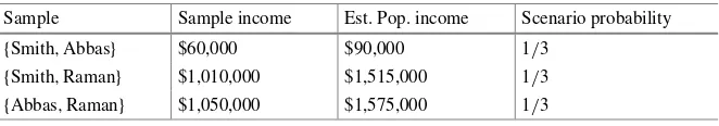
Table 1 Possible scenarios, along with probabilities, for a sampling and estimation exercise
Sample Sample income Est. Pop. income Scenario probability
{Smith,Abbas} $60,000 $90,000 1/3
{Smith,Raman} $1,010,000 $1,515,000 1/3 {Abbas,Raman} $1,050,000 $1,575,000 1/3
$1,000,000. The total income for this population is $1,060,000. If we take anSRS
of sizek=2—and hence estimate the income for the population as 1.5 times the income for the sampled individuals—then the outcome of our sampling and esti-mation exercise would follow one of the scenarios given in Table1. Each of the scenarios is equally likely, and the expected value (also called the “mean value”) of our estimate is computed as
expected value=(1/3)·(90,000)+(1/3)·(1,515,000)+(1/3)·(1,575,000)
=1,060,000,
which is equal to the true answer. In general, it is important to evaluate the accuracy (degree of systematic error) and precision (degree of variability) of a sampling and estimation scheme. Thebias, i.e., expected error, is a common measure of accuracy, and, for estimators with low bias, thestandard erroris a common measure of pre-cision. The bias of our income estimator is 0 and the standard error is computed as the square root of thevariance(expected squared deviation from the mean) of our estimator:
SE=(1/3)·(90,000−1,060,000)2+(1/3)·(1,515,000−1,060,000)2
+(1/3)·(1,575,000−1,060,000)21/2≈687,000.
For more complicated population parameters and their estimators, there are often no simple formulas for gauging accuracy and precision. In these cases, one can some-times resort to techniques based onsubsampling, that is, taking one or more random samples from the initial population sample. Well known subsampling techniques for estimating bias and standard error include the “jackknife” and “bootstrap” methods; see [6]. In general, the accuracy and precision of a well designed sampling-based es-timator should increase as the sample size increases. We discuss these issues further in Sect.4.
1.2 Database Sampling
• Scarce versus ubiquitous data.In the classical setting, samples are usually ex-pensive to obtain and data is hard to come by, and so sample sizes tend to be small. In database sampling, the population size can be enormous (terabytes of data), and samples are relatively easy to collect, so that sample sizes can be rel-atively large [7,8]. The emphasis in the database setting is on the sample as a flexible, lossy, compressed synopsis of the data that can be used to obtain quick approximate answers to user queries.
• Different sampling schemes. As a consequence of the complex storage for-mats and retrieval mechanisms that are characteristic of modern database sys-tems, many sampling schemes that were unknown or of marginal interest in the classical setting are central to database sampling. For example, the classical lit-erature pays relatively little attention to Bernoulli sampling schemes (described in Sect.2.1below), but such schemes are very important for database sampling because they can be easily parallelized across data partitions [9,10]. As another example, tuples in a relational database are typically retrieved from disk in units of pages or extents. This fact strongly influences the choice of sampling and es-timation schemes, and indeed has led to the introduction of several novel meth-ods [11–13]. As a final example, estimates of the answer to an aggregation query involving select–project–join operations are often based on samples drawn indi-vidually from the input base relations [14,15], a situation that does not arise in the classical setting.
• No domain expertise.In the classical setting, sampling and estimation are often carried out by an expert statistician who has prior knowledge about the population being sampled. As a result, the classical literature is rife with sampling schemes that explicitly incorporate auxiliary information about the population, as well as “model-based” schemes [4, Chap. 5] in which the population is assumed to be a sample from a hypothesized “super-population” distribution. In contrast, database systems typically must view the population (i.e., the database) as a black box, and so cannot exploit these specialized techniques.
• Auxiliary synopses.In contrast to a classical statistician, a database designer of-ten has the opportunity to scan each population element as it enters the system, and therefore has the opportunity to maintain auxiliary data synopses, such as an index of “outlier” values or other data summaries, which can be used to increase the precision of sampling and estimation algorithms. If available, knowledge of the query workload can be used to guide synopsis creation; see [16–23] for ex-amples of the use of workloads and synopses to increase precision.
as a precursor to modern data-stream sampling techniques. Online-aggregation al-gorithms take, as input, streams of data generated by random scans of one or more (finite) relations, and produce continually-refined estimates of answers to aggre-gation queries over the relations, along with precision measures. The user aborts the query as soon as the running estimates are sufficiently precise; although the data stream is finite, query processing usually terminates long before the end of the stream is reached. Recent work on database sampling includes extensions of online aggregation methodology [39–42], application of bootstrapping ideas to facilitate approximate answering of very complex aggregation queries [43], and development of techniques for sampling-based discovery of correlations, functional dependen-cies, and other data relationships for purposes of query optimization and data inte-gration [9,44–46].
Collective experience has shown that sampling can be a very powerful tool, pro-vided that it is applied judiciously. In general, sampling is well suited to very quickly identifying pervasive patterns and properties of the data when a rough approxima-tion suffices; for example, industrial-strength sampling-enhanced query engines can speed up some common decision-support queries by orders of magnitude [10]. On the other hand, sampling is poorly suited for finding “needles in haystacks” or for producing highly precise estimates. The needle-in-haystack phenomenon appears in numerous guises. For example, precisely estimating the selectivity of a join that re-turns very few tuples is an extremely difficult task, since a random sample from the base relations will likely contain almost no elements of the join result [16,31].2As another example, sampling can perform poorly when data values are highly skewed. For example, suppose we wish to estimate the average of the values in a data set that consists of 106 values equal to 1 and five values equal to 108. The five
out-lier values are the needles in the haystack: if, as is likely, these values are not in-cluded in the sample, then the sampling-based estimate of the average value will be low by orders of magnitude. Even when the data is relatively well behaved, some population parameters are inherently hard to estimate from a sample. One notori-ously difficult parameter is the number of distinct values in a population [47,48]. Problems arise both when there is skew in the data-value frequencies and when there are many data values, each appearing a small number of times. In the for-mer scenario, those values that appear few times in the database are the needles in the haystack; in the latter scenario, the sample is likely to contain no dupli-cate values, in which case accurate assessment of a scale-up factor is impossible. Other challenging population parameters include the minimum or maximum data value; see [49]. Researchers continue to develop new methods to deal with these problems, typically by exploiting auxiliary data synopses and workload informa-tion.
1.3 Sampling from Data Streams
Data-stream sampling problems require the application of many ideas and tech-niques from traditional database sampling, but also need significant new innova-tions, especially to handle queries over infinite-length streams. Indeed, the un-bounded nature of streaming data represents a major departure from the traditional setting. We give a brief overview of the various stream-sampling techniques consid-ered in this chapter.
Our discussion centers around the problem of obtaining a sample from a win-dow, i.e., a subinterval of the data stream, where the desired sample size is much smaller than the number of elements in the window. We draw an important distinc-tion between astationarywindow, whose endpoints are specified times or specified positions in the stream sequence, and aslidingwindow whose endpoints move for-ward as time progresses. Examples of the latter type of window include “the most recentnelements in the stream” and “elements that have arrived within the past hour.” Sampling from a finite stream is a special case of sampling from a station-ary window in which the window boundaries correspond to the first and last stream elements. When dealing with a stationary window, many traditional tools and tech-niques for database sampling can be directly brought to bear. In general, sampling from a sliding window is a much harder problem than sampling from a stationary window: in the former case, elements must be removed from the sample as they expire, and maintaining a sample of adequate size can be difficult. We also consider “generalized” windows in which the stream consists of a sequence of transactions that insert and delete items into the window; a sliding window corresponds to the special case in which items are deleted in the same order that they are inserted.
Much attention has focused onSRSschemes because of the large body of existing
theory and methods for inference from anSRS; we therefore discuss such schemes in detail. We also consider Bernoulli sampling schemes, as well as stratified schemes in which the window is divided into equal disjoint segments (the strata) and anSRS
of fixed size is drawn from each stratum. As discussed in Sect.2.3below, stratified sampling can be advantageous when the data stream exhibits significant autocor-relation, so that elements close together in the stream tend to have similar values. The foregoing schemes fall into the category ofequal-probability samplingbecause each window element is equally likely to be included in the sample. For some ap-plications it may be desirable to bias a sample toward more recent elements. In the following sections, we discuss both equal-probability and biased sampling schemes.
2 Sampling from a Stationary Window
We consider a stationary window containingnelementse1, e2, . . . , en, enumerated
in arrival order. If the endpoints of the window are defined in terms of time points t1andt2, then the numbernof elements in the window is possibly random; this fact
sampling from the window is worthwhile. We briefly discuss Bernoulli sampling schemes in which the size of the sample is random, but devote most of our attention to sampling techniques that produce a sample of a specified size.
2.1 Bernoulli Sampling
ABernoullisampling scheme with sampling rateq∈(0,1)includes each element in the sample with probabilityq and excludes the element with probability 1−q, independently of the other elements. This type of sampling is also called “bino-mial” sampling because the sample size is binomially distributed so that the prob-ability that the sample contains exactlyk elements is equal to nkqk(1−q)n−k. The expected size of the sample isnq. It follows from the central limit theorem for independent and identically distributed random variables [50, Sect. 27] that, for example, whennis reasonably large andq is not vanishingly small, the deviation from the expected size is within±100ε% with probability close to 98 %, where ε=2√(1−q)/nq. For example, if the window contains 10,000 elements and we draw a 1 % Bernoulli sample, then the true sample size will be between 80 and 120 with probability close to 98 %. Even though the size of a Bernoulli sample is ran-dom, Bernoulli sampling, likeSRSandSRSWR, is auniform sampling scheme, in that any two samples of the same size are equally likely to be produced.
Bernoulli sampling is appealingly easy to implement, given a pseudorandom number generator [51, Chap. 7]. A naive implementation generates for each ele-mentei a pseudorandom numberUi uniformly distributed on[0,1]; elementei is
included in the sample if and only ifUi ≤q. A more efficient implementation uses
the fact that the number of elements that are skipped between successive inclusions has a geometric distribution: ifi is the number of elements skipped afterei is
in-cluded, then Pr{i =j} =q(1−q)j for j ≥0. To saveCPUtime, these random
skips can be generated directly. Specifically, ifUi is a random number distributed
uniformly on[0,1], theni = ⌊logUi/log(1−q)⌋has the foregoing geometric
distribution, where⌊x⌋denotes the largest integer less than or equal tox; see [51, p. 465]. Figure1displays the pseudocode for the resulting algorithm, which is exe-cuted whenever a new elementei arrives. Lines 1–4 represent an initialization step
that is executed upon the arrival of the first element (i.e., whenm=0 andi=1). Observe that the algorithm usually does almost nothing. The “expensive” calls to the pseudorandom number generator and the log() function occur only at element-inclusion times. As mentioned previously, another key advantage of the foregoing algorithm is that it is easily parallelizable over data partitions.
A generalization of the Bernoulli sampling scheme uses a different inclusion probability for each element, including elementiin the sample with probabilityqi.
//qis the Bernoulli sampling rate
//eiis the element that has just arrived (i≥1)
//mis the index of the next element to be included (static variable initialized to 0) //Bis the Bernoulli sample of stream elements (initialized to∅)
//is the size of the skip
//random()returns a uniform[0,1] pseudorandom number
1 ifm=0then //generate initial skip 2 U←random()
3 ← ⌊logU/log(1−q)⌋
4 m←+1 //compute index of first element to insert 5 ifi=mthen //insert element into sample and generate skip 6 B←B∪ {ei}
7 U←random()
8 ← ⌊logU/log(1−q)⌋
9 m←m++1 //update index of next element to insert
Fig. 1 An algorithm for Bernoulli sampling
The main drawback of both Bernoulli and Poisson sampling is the uncontrollable variability of the sample size, which can become especially problematic when the desired sample size is small. In the remainder of this section, we focus on sampling schemes in which the final sample size is deterministic.
2.2 Reservoir Sampling
The reservoir sampling algorithm of Waterman [52, pp. 123–124] and McLeod and Bellhouse [53] produces anSRSofkelements from a window of lengthn, wherek is specified a priori. The idea is to initialize a “reservoir” ofkelements by inserting elementse1, e2, . . . , ek. Then, fori=k+1, k+2, . . . , n, elementei is inserted in
the reservoir with a specified probabilitypi and ignored with probability 1−pi;
an inserted element overwrites a “victim” that is chosen randomly and uniformly from thekelements currently in the reservoir. We denote bySj the set of elements
in the reservoir just after elementej has been processed. By convention, we take
p1=p2= · · · =pk=1. If we can choose thepi’s so that, for eachj, the setSj is
anSRSfromUj= {e1, e2, . . . , ej}, then clearlySnwill be the desired final sample.
The probability thatei is included in anSRSfromUiequalsk/ i, and so a plausible
choice for the inclusion probabilities is given bypi=k/(i∨k)for 1≤i≤n.3The
following theorem asserts that the resulting algorithm indeed produces anSRS.
Theorem 1(McLeod and Bellhouse [53]) In the reservoir sampling algorithm with pi=k/(i∨k)for1≤i≤n,the setSjis a simple random sample of sizej∧kfrom
Uj= {e1, e2, . . . , ej}for each1≤j≤n.
3Throughout, we denote byx
Proof The proof is by induction onj. The assertion of the theorem is obvious for
where the second equality follows from the induction hypothesis and the indepen-dence of the two given events. Now suppose thatej∈A. Forer∈Uj−1−A, letAr
Efficient implementation of reservoir sampling is more complicated than that of Bernoulli sampling because of the more complicated probability distribution of the number of skips between successive inclusions. Specifically, denoting byi
the number of skips before the next inclusion, given that elementei has just been
included, we have efficient algorithm for generating samples from the above distribution. For small values ofi, the fastest way to generate a skip is to use the method ofinversion: if Fi−1(x)=min{m: Fi(m)≥x}andU is a random variable uniformly distributed
on[0,1], then it is not hard to show that the random variableX=Fi−1(U )has the desired distribution functionFi, as doesX′=Fi−1(1−U ); see [51, Sect. 8.2.1]. For
to generate sample values, along with a constantci—greater than 1 but as close to
1 as possible—such thatfi(⌊x⌋)≤cigi(x)for allx≥0. IfXis a random variable
with density functiongandUis a uniform random variable independent ofX, then Pr{⌊X⌋ ≤x|U≤fi(⌊X⌋)/cigi(X)} =Fi(x). That is, if we generate pairs(X, U )
until the relation U≤fi(⌊X⌋)/cigi(X)holds, then the final random variableX,
after truncation to the nearest integer, has the desired distribution functionFi. It can
be shown that, on average,cipairs(X, U )need to be generated to produce a sample
fromFi. As a further refinement, we can reduce the number of expensive evaluations
of the functionfiby finding a functionhi“close” tofisuch thathiis inexpensive to
evaluate andhi(x)≤fi(x)forx≥0. Then, to test whetherU≤fi(⌊X⌋)/cigi(X),
we first test (inexpensively) whetherU≤hi(⌊X⌋)/cigi(X). Only in the rare event
that this first test fails do we need to apply the expensive original test. This trick is sometimes called the “squeeze” method. Vitter shows that an appropriate choice for ci isci=(i+1)/(i−k+1), with corresponding choices density functiongi. Thus it is indeed easy to generate sample values fromgi.
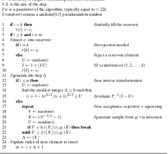
Figure2displays the pseudocode for the overall algorithm; see [54] for a perfor-mance analysis and some further optimizations.4 As with the algorithm in Fig.1, the algorithm in Fig.2is executed whenever a new elementei arrives.
Observe that the insertion probability pi =k/(i∨k)decreases as i increases
so that it becomes increasingly difficult to insert an element into the reservoir. On the other hand, the number of opportunities for an inserted elementei to be
sub-sequently displaced from the sample by an arriving element also decreases as i increases. These two opposing trends precisely balance each other at all times so that the probability of being in the final sample is the same for all of the elements in the window.
Note that the reservoir sampling algorithm does not require prior knowledge ofn, the size of the window—the algorithm can be terminated after any arbitrary number of elements have arrived, and the contents of the reservoir are guaranteed to be an
SRS of these elements. If the window size is known in advance, then a variation
of reservoir sampling, calledsequential sampling, can be used to obtain the desired
SRSof sizekmore efficiently. Specifically, reservoir sampling has a time complexity ofO(k+klog(n/ k))whereas sequential sampling has a complexity ofO(k). The
//kis the size of the reservoir andnis the number of elements in the window //eiis the element that has just arrived (i≥1)
//mis the index of the next element≥ekto be included (static variable initialized tok) //ris an array of lengthkcontaining the reservoir elements
//is the size of the skip
//αis a parameter of the algorithm, typically equal to≈22k //random()returns a uniform[0,1] pseudorandom number
1 ifi < kthen //initially fill the reservoir 2 r[i] ←ei
12 ifi≤αthen //use inverse transformation
13 U←random()
14 find the smallest integer≥0 such that 15 (i+1−k)+1/(i
24 //update index of next element to insert 25 m←i++1
Fig. 2 Vitter’s algorithm for reservoir sampling
sequential-sampling algorithm, due to Vitter [55], is similar in spirit to reservoir sampling, and is based on the observation that
˜
where˜ij is the number of skips before the next inclusion, given that elementen−j
has just been included in the sample and that the sample size just after the inclusion ofen−j is|S| =k−i. Herexn denotes the falling powerx(x−1)· · ·(x−n+1).
arriving element into the sample, and (iv) setsi←i−1 andj ←j − ˜ij−1.
Steps (i)–(iv) are repeated untili=0.
At each execution of Step (i), the specific method used to generate˜ij depends
upon the current values of i and j, as well as algorithmic parameters α and β. Specifically, ifi≥αj, then the algorithm generates˜ij by inversion, similarly to
lines 13–15 in Fig.2. Otherwise, the algorithm generates˜ij using acceptance–
rejection and squeezing, exactly as in lines 17–23 in Fig.2, but using either c1=
j/(j−i+1),
i2/j > β, respectively. The values ofαandβ are implementation dependent; Vitter foundα=0.07 andβ=50 optimal for his experiments, but also noted that setting β≈1 minimizes the average number of random numbers generated by the algo-rithm. See [55] for further details and optimizations.5
2.3 Other Sampling Schemes
We briefly mention several other sampling schemes, some of which build upon or incorporate the reservoir algorithm of Sect.2.2.
Stratified Sampling
As mentioned before, a stratified sampling scheme divides the window into disjoint intervals, or strata, and takes a sample of specified size from each stratum. The
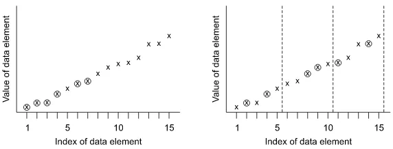
Fig. 3 (a) A realization of reservoir sampling (sample size=6). (b) A realization of stratified sampling (sample size=6)
simplest scheme specifies strata of approximately equal length and takes a fixed size random sample from each stratum using reservoir sampling; the random samples are of equal size.
When elements close together in the stream tend to have similar values, then the values within each stratum tend to be homogeneous so that a small sample from a stratum contains a large amount of information about all of the elements in the stra-tum. Figures3(a) and3(b) provide another way to view the potential benefit of strat-ified sampling. The window comprises 15 real-valued elements, and circled points correspond to sampled elements. Figure3(a) depicts an unfortunate realization of an SRS: by sheer bad luck, the early, low-valued elements are disproportionately
represented in the sample. This would lead, for example, to an underestimate of the average value of the elements in the window. Stratified sampling avoids this bad sit-uation: a typical realization of a stratified sample (with three strata of length 5 each) might look as in Fig.3(b). Observe that elements from all parts of the window are well represented. Such a sample would lead, e.g., to a better estimate of the average value.
Deterministic and Semi-Deterministic Schemes
Of course, the simplest scheme for producing a sample of sizekinserts everymth el-ement in the window into the sample, wherem=n/ k. There are two disadvantages to this approach. First, it is not possible to draw statistical inferences about the entire window from the sample because the necessary probabilistic context is not present. In addition, if the data in the window are periodic with a frequency that matches the sampling rate, then the sampled data will be unrepresentative of the window as a whole. For example, if there are strong weekly periodicities in the data and we sample the data every Monday, then we will have a distorted picture of the data val-ues that appear throughout the week. One way to ameliorate the former problem is to usesystematic sampling[1, Chap. 8]. To effect this scheme, generate a random numberL between 1 andm. Then insert elements eL, eL+m, eL+2m, . . . , en−m+L
remains—in the presence of periodicity, estimators based on systematic sampling can have large standard errors. On the other hand, if the data are not periodic but exhibit a strong trend, then systematic sampling can perform very well because, like stratified sampling, systematic sampling ensures that the sampled elements are spread relatively evenly throughout the window. Indeed, systematic sampling can be viewed as a type of stratified sampling where theith stratum comprises elements e(i−1)m+1, e(i−1)m+2, . . . , eimand we sample one element from each stratum—the
sampling mechanisms for the different strata are completely synchronized, however, rather than independent as in standard stratified sampling.
Biased Reservoir Sampling
Consider a generalized reservoir scheme in which the sequence of inclusion proba-bilities{pi: 1≤i≤n}either is nondecreasing or does not decrease as quickly as
the sequence{k/(i∨k): 1≤i≤n}. This version of reservoir sampling favors in-clusion of recently arrived elements over elements that arrived earlier in the stream. As illustrated in Sect.4.4below, it can be useful to compute the marginal proba-bility that a specified elementei belongs to the final sampleS. The probability that
ei is selected for insertion is, of course, equal topi. Forj > i∨k, the probability
θij thateiis not displaced from the sample when elementej arrives equals the
prob-ability thatej is not selected for insertion plus the probability thatej is selected but
does not displaceei. Ifj≤k, then the processing ofej cannot result in the removal
ofeifrom the reservoir. Thus
θij=(1−pj)+pj
ifj > k, andθij=1 otherwise. Because the random decisions made at the
succes-sive steps of the reservoir sampling scheme are mutually independent, it follows that the probability thatei is included inSis the product of the foregoing probabilities:
Pr{ei∈S} =pi
Similar arguments lead to formulas for joint inclusion probabilities: settingαi,j =
Thus the probability that elementei is in the final sample decreases geometrically
asidecreases; the larger the value ofp, the faster the rate of decrease.
Chao [56] has extended the basic reservoir sampling algorithm to handle arbitrary sampling probabilities. Specifically, just after the processing of elementei, Chao’s
scheme ensures that the inclusion probabilities satisfy Pr{ej∈S} ∝rj for 1≤j≤i,
where{rj: j≥1}is a prespecified sequence of positive numbers. The analysis of
this scheme is rather complicated, and so we refer the reader to [56] for a complete discussion.
Biased Sampling by Halving
Another way to obtain a biased sample of size k is to divide the window intoL strata ofm=n/Lelements each, denotedΛ1, Λ2, . . . , ΛL, and maintain a running
sampleSof sizekas follows. The sample is initialized as anSRSof sizekfromΛ1;
(unbiased) reservoir sampling or sequential sampling may be used for this purpose. At thejth subsequent step,k/2 randomly-selected elements ofSare overwritten by the elements of anSRSof sizek/2 fromΛj+1(so that half of the elements inSare
purged). For an elementei∈Λj, we have, after the procedure has terminated,
Pr{ei∈S} =
k m
1 2
L−(j∨2)+1
.
As with biased reservoir sampling, the halving scheme ensures that the probabil-ity thatei is in the final samples falls geometrically asidecreases. Brönnimann et
al. [57] describe a related scheme when each stream element is ad-vector of 0–1 data that represents, e.g., the presence or absence in a transaction of each ofditems. In this setting, the goal of each halving step is to create a subsample in which the relative occurrence frequencies of the items are as close as possible to the corre-sponding frequencies over all of the transactions in the original sample. The scheme uses a deterministic halving method called “epsilon approximation” to achieve this goal. The relative item frequencies in subsamples produced by this latter method tend to be closer to the relative frequencies in the original sample than are those in subsamples obtained bySRS.
3 Sampling from a Sliding Window
whereas a timestamp-based window of lengtht contains all elements that arrived within the pastttime units. Because a sliding window inherently favors recently ar-rived elements, we focus on techniques for equal-probability sampling from within the window itself. For completeness, we also provide a brief discussion of general-izedwindows in which elements need not leave the window in arrival order.
3.1 Sequence-Based Windows
We consider windows {Wj: j ≥1}, each of length n, where Wj = {ej, ej+1,
. . . , ej+n−1}. A number of algorithms have been proposed for producing, for each
windowWj, anSRSSj ofkelements fromWj. The major difference between the
algorithms lies in the tradeoff between the amount of memory required and the de-gree of dependence between the successiveSj’s.
Complete Resampling
At one end of the spectrum, a “complete resampling” algorithm takes an indepen-dent sample from eachWj. To do this, the set of elements in the current window is
buffered in memory and updated incrementally, i.e.,Wj+1is obtained fromWj by
deletingej and insertingej+n. Reservoir sampling (or, more efficiently, sequential
sampling) can then be used to extractSj fromWj. TheSj’s produced by this
algo-rithm have the desirable property of being mutually independent. This algoalgo-rithm is impractical, however, because it has memory andCPUrequirements ofO(n), andn is assumed to be very large.
A Passive Algorithm
At the other end of the spectrum, the “passive” algorithm described in [58] obtains anSRSof sizekfrom the firstnelements using reservoir sampling. Thereafter, the sample is updated only when the arrival of an element coincides with the expiration of an element in the sample, in which case the expired element is removed and the new element is inserted. An argument similar to the proof of Theorem1shows that eachSjis aSRSfromWj. Moreover, the memory requirement isO(k), the same as
for the stationary-window algorithms. In contrast to complete resampling, however, the passive algorithm producesSj’s that are highly correlated. For example,Sj and
Sj+1are identical or almost identical for eachj. Indeed, if the data elements are
periodic with periodn, then everySj is identical toS1; this assertion follows from
the fact that if elementei is in the sample, then so isei+j n forj ≥1. Thus ifS1is
not representative, e.g., the sampled elements are clustered withinW1as in Fig.3(a),
Subsampling from a Bernoulli Sample
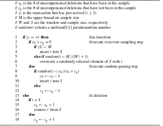
Babcock et al. [58] provide two algorithms intermediate to those discussed above. The first algorithm inserts elements into a setBusing a Bernoulli sampling scheme; elements are removed fromB when, and only when, they expire. The algorithm tries to ensure that the size ofBexceedskat all times by using an inflated Bernoulli sampling rate ofq=(2cklogn)/n, wherecis a fixed constant. Each final sample Sj is then obtained as a simple random subsample of sizekfromB. An argument
using Chernoff bounds (see, e.g., [59]) shows that the size ofBlies betweenkand 4cklognwith a probability that exceeds 1−O(n−c). TheSj’s are less dependent
than in the passive algorithm, but the expected memory requirement isO(klogn). Also observe that ifBj is the size ofB afterj elements have been processed and
ifγ (i)denotes the index of theith step at which the sample size either increases or decreases by 1, then Pr{Bγ (i)+1=Bγ (i)+1} =Pr{Bγ (i)+1=Bγ (i)−1} =1/2. That
is, the process{Bγ (i): i≥0}behaves like a symmetric random walk. It follows that,
with probability 1, the size of the Bernoulli sample will fall belowkinfinitely often, which can be problematic if sampling is performed over a very long period of time.
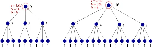
Chain Sampling
The second algorithm, calledchain sampling, retains the improved independence properties of theSj’s relative to the passive algorithm, but reduces the expected
memory requirement toO(k). The basic algorithm maintains a sample of size 1, and a sample of size k is obtained by runningk independent chain-samplers in parallel. Observe that the overall sample is therefore a simple random sample with replacement—we discuss this issue after we describe the algorithm.
To maintain a sampleS of size 1, the algorithm initially inserts each newly ar-rived elementei into the sample (i.e., sets the sample equal toS= {ei}) with
prob-ability 1/ i for 1≤i≤n. Thus the algorithm behaves initially as a reservoir sam-pler so that, after thenth element has been observed,S is anSRS of size 1 from {e1, e2, . . . , en}. Subsequently, whenever elementei arrives and, just prior to arrival,
the sample isS= {ej}withi=j+n(so that the sample elementej expires), an
el-ement randomly and uniformly selected from amongej+1, ej+2, . . . , ej+nbecomes
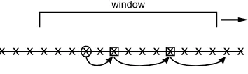
the new sample element. Observe that the algorithm does not need to store all of the elements in the window in order to replace expiring sample elements—it suffices to store a “chain” of elements associated with the sample, where the first element of the chain is the sample itself; see Fig.4. In more detail, whenever an element ei is added to the chain, the algorithm randomly selects the indexK of the
ele-menteK that will replaceei upon expiration. IndexK is uniformly distributed on
i+1, i+2, . . . , i+n, the indexes of the elements that will be in the window just afterei expires. When elementeK arrives, the algorithm storeseK in memory and
randomly selects the indexMof the element that will replaceeKupon expiration.
Fig. 4 Chain sampling (sample size=1).Arrowspoint to the elements of the current chain, thecircled elementrepresents the current sample, andelements within squaresrepresent those elements of the chain currently stored in memory
reservoir sampling mechanism. Specifically, suppose that elementei arrives and,
just prior to arrival, the sample isS= {ej}withi < j+n(so that the sample element
ej does not expire). Then, with probability 1/n, elementeibecomes the sample
ele-ment; the previous sample elementejand its associated chain are discarded, and the
algorithm starts to build a new chain for the new sample element. With probability 1−(1/n), elementej remains as the sample element and its associated chain is not
discarded. To see that this procedure is correct wheni < j +n, observe that just prior to the processing ofei, we can viewSas a reservoir sample of size 1 from the
“stream” ofn−1 elements given by ei−n+1, ei−n+2, . . . , ei−1. Thus, addingei to
the sample with probability 1/namounts to executing a step of the usual reservoir algorithm, so that, after processingei, the setSremains anSRSof size 1 from the
updated windowWi−n+1= {ei−n+1, ei−n+2, . . . , ei}. Because the SRSproperty of
S is preserved at each arrival epoch whether or not the current sample expires, a straightforward induction argument formally establishes thatS is anSRSfrom the current window at all times.
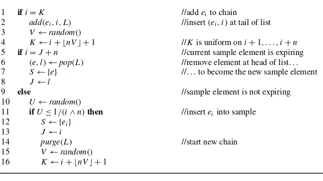
Figure5 displays the pseudocode for the foregoing algorithm; the code is ex-ecuted whenever a new elementei arrives. In the figure, the variableLdenotes a
linked list of chained elements of the form(e, l), wheree is an element andl is the element’s index in the stream; the list does not contain the current sample ele-ment, which is stored separately inS. Elements appear from head to tail in order of arrival, with the most recently arrived element at the tail of the list. The functions add,pop, andpurgeadd a new element to the tail of the list, remove (and return the value of) the element at the head of the list, and remove all elements from the list, respectively.
We now analyze the memory requirements of the algorithm by studying the max-imum amount of memory consumed during the evolution of a single chain.6Denote byMthe total number of elements inserted into memory during the evolution of the chain, including the initial sample. ThusM≥1 andM is an upper bound on the maximum memory actually consumed because it ignores decreases in memory con-sumption due to expiration of elements in the chain. Denote byXthe distance from the initial sample to the next element in the chain, and recall thatX is uniformly distributed on{1,2, . . . , n}. Observe thatM≥2 if and only ifX < nand, after the
6See [58] for an alternative analysis. Whenever an arriving elemente
//nis the number of elements in the window //eiis the element that has just arrived (i≥1)
//Lis a linked list (static) of chained elements (excluding sample) of the form(e, l) //Sis the sample (static, contains exactly one element)
//Jis the index of the element in the sample (static, initialized to 0)
//Kis the index of the next element to be added to the chain (static, initialized to 0) //random()returns a uniform[0,1] pseudorandom number
1 ifi=K //addeito chain
2 add(ei, i, L) //insert(ei, i)at tail of list 3 V←random()
4 K←i+ ⌊nV⌋ +1 //Kis uniform oni+1, . . . , i+n
5 ifi=J+n //current sample element is expiring
6 (e, l)←pop(L) //remove element at head of list. . . 7 S← {e} //. . .to become the new sample element
8 J←l
9 else //sample element is not expiring
10 U←random()
Fig. 5 Chain-sampling algorithm (sample size=1)
initial sample, none of the nextX arriving elements become the new sample ele-ment. Thus Pr{M≥2|M≥1, X=j} ≤(1−n−1)jfor 1≤j≤n. Unconditioning
Moreover, forj =αlnnwithαa fixed positive constant, we have
Pr{M≥j+1} =ejlnβ=n−c,
Fig. 6 Stratified sampling for a sliding window (n=12,m=4,k=2). Thecircled elementslying within the window represent the members of the current sample, andcircled elementslying to the left of the window represent former members of the sample that have expired
As mentioned previously, chain sampling produces anSRSWRrather than anSRS. One way of dealing with this issue is increase the size of the initialSRSWRsample
S′to|S′| =k+α, whereαis large enough so that, after removal of duplicates, the size of the finalSRSSwill equal or exceedkwith high probability. Subsampling can be then be used, if desired, to ensure that the final sample size|S|equalskexactly. Using results on “occupancy distributions” [60, p. 102] it can be shown that
Pr|S|< k=
and a value of α that makes the right side sufficiently small can be determined numerically, at least in principle. Assuming thatk < n/2, a conservative but simpler approach ensures that Pr{|S|< k}< n−c for a specified constantc≥1 by setting
This assertion follows from a couple of simple bounding arguments.7
Stratified Sampling
The stratified sampling scheme for a stationary window can be adapted to obtain a stratified sample from a sliding window. The simplest scheme divides the stream into strata of lengthm, wheremdivides the window lengthn; see Fig.6. Reservoir sampling is used to obtain aSRSof sizek < mfrom each stratum. Sampled elements expire in the usual manner. The current window always contains betweenlandl+1 strata, wherel=n/m, and all but perhaps the first and last strata are of equal length,
7We deriveα