Australian Journal of Basic and Applied Sciences, 5(3): 28-37, 2011 ISSN 1991-8178
Corresponding Author:F.A.M. Elfaki, Department of Science in Engineering, Kulliyyah of Engineering, IIUM Jalan
Statistical Process Control For Failure Crushing Time Data Using
Competing Risks Model
1
F.A.M. Elfaki,
1J. Daud,
1M. Azram,
2Bin Daud. I,
2N.A. Ibrahim and
3M. Usman
1
Department of Science in Engineering, Kulliyyah of Engineering, IIUM Jalan Gombak, 50728,
Kuala Lumpur, Malaysia.
2
Department of Mathematics, Faculty of Science and Environmental Studies University Putra
Malaysia, 43400, Serdang, Selangor.
3
Faculty of Economics, Universitas Malahayati, Ji. Pramuka No. 27 Kemiling Bandar Lampung,
Indonesia
Abstract: This paper describes a Statistical Process Control (SPC) for failure crushing time data using competing risks model. The model is based on the widely known proportional hazard regression model for a variety of censoring. A competing risks model identifies the set of possible failed components given the true cause of failure. EM algorithm method is used to estimate the parameter of the model. The results of this study show that, the competing risks model performs well for SPC using SAS software.
Key words: SPC; Competing Risks; Cox’s Model; Reliability; EM algorithm.
INTRODUCTION
Statistical Process Control (SPC) is a branch of the larger field of quality control, aims at controlling the quality of the items produced in an ongoing processes. SPC is a powerful collection of problem-solving tools useful in achieving process stability and improving capability through the reduction of variability (Montgomery, 1985; 1991). SPC also, is the application of statistical principles and techniques in all stages of production directed toward the most economical manufacturing of a product. Moreover, SPC involves the use of statistical analyses to evaluate and monitor process performance. These techniques identify the existence of special or common causes that affect the process performance. Common causes are inherent to the process, variations and interaction of the people, machines, raw materials, and the process, whereas special causes are due to some abnormality that prevents operational stability. General introductions to SPC methods are given in Montgomery (1985), Kane (1986), Rado (1989), Besterfield (1986), Grant and Leavenworth (1980), Dhillon (1985), Duncan (1974), Wadsworth, Stephens and Godfrey (1986), Ryan (1989), Stoumbos (2002), Chou et all (1990), Stuart et al (1996), Parlar and Wesolowsky (1999), Nedumaran and Pignatiello (2001), Gunter (1989), Clements (1989), Spiring (1991), Chan et al (1988) and Xie et al (2002).
The most important tool in SPC is the control chart and process capability index. There are two basic types of control charts: charts for variables data and charts for attributes data. Variable data control charts are useful when the parameter of interest can be conveniently measured numerically, for example, the measurement of the diameter of a cylindrical part. Whereas attribute data control chart are useful when the parameter of interest cannot be conveniently measured numerically, for example, the inspection of the finished surface of a cylindrical part. and R charts belong to the category of variable data charts, and p and c charts belongx to the category of attribute data charts.
capability), and variability across the (long-term process capability). It is particularly helpful if the data for a process capability study are collected in two to three different time periods, such as different shift and different day’s. The variable control charts are important in the quality program of many industries, their ability to identify process improvement opportunities.
The theory of competing risks is applied in the analysis of reliability and survival data involving several different failure types or risks. In an industry, for instance, one might distinguish between a mechanical device failure attributable to a component that has failed and those due to unrelated causes. This constitutes the different risks under consideration. Typically, the data include the time of failure or censoring of each individual, as well as an indicator of the type of failures. To assess the effects of covariates on cause-specific hazards, one can perform a parametric Cox’s proportional hazards model, treating failure types which are of interest as censored observation (Aly, et al., 1994; Cheng et al., 1998).
In this paper, we use competing risks model that is, parametric Cox’s model with Weibull distribution based on EM algorithm, to examine the state of control of the process, that is, variable control charts, and estimation of capability indices. However, the parameters are obtained by using SAS software.
2. Statistical Process Control:
The goal of statistical process control (SPC) is to ensure that a process, with outputs that exhibit both systematic and random components, produces high quality items over time. To do so a process must be stable and consistent, with a steady systematic component and with a typical random component small enough not to seriously degrade item quality. (This is to say that the control limits should define an acceptable range of measurements to ensure adequate product quality). Because the random component causes the sequence of measurements to vary, process observers must try to distinguish between ordinary fluctuations (which require not intervention), and aberrant behavior (which must be corrected or at least understood). Control charts and process capability index based on competing risks model provide an objective way to do this.
Section 2.1 discusses control charts and section 2.3 discusses statistical process control concepts of capability.
2.1. The x Chart
The control chart is a simple graphic procedure to study the state of the process. The control chart isx a time-ordered sequences of observations of data of interest plotted between two horizontal lines called the control limits, the upper control limit (UCL), and lower control limit (LCL). Periodically, such as every hour, a sample of say n items from the production process are picked and the sample average (denoted by ) isx plotted on the vertical axis. This process is continued and the consecutive points are joined by a straight line. If any point falls between the limits the process is said to be under statistical control. If a single observation lies beyond the control limits, the process is declared to be out of control and corrective action is taken to detect and eliminate the assignable cause. In general, the center line, the upper control limit, and the lower control limit are defined as:
2.2 The R Control Chart:
Plotting values of the sample range R on a control chart may monitor process variability. The center line and control limits of the R chart are as follows:
(4)
The constants D3 and D4 are tabulated for various values of n Appendix of Montgomery (1989). 2.3. Process Capability:
Data built up over a period of using control charts in the way described may be used to know how the process ought to behave through the assessment of its capability, that is, its capacity to meet customer’s or other specifications. A review of historical control charts will establish the degree of statistical control of the process and may also be used as a basis for estimating mean μ and standard deviation σ. Following this, the ability of the process to meet specification is assessed through calculation of one or more capability indices. In practice, the values of μ and σ usually are not known. The process must be stable in order to produce reliable estimates of μ and σ. Assuming that the process has reached a state of statistical control, the question often arises as to whether it can meet the tolerance.
The most commonly used measures of process capability are CP, CPU CPL and Cpk. These indices have
been utilized by a number of Japanese companies and in the U.S. automotive industry (Kane, 1986). Several researches used process capability in their studies such as, Kane (1986) who describes a distribution of a function of Cp. Specifically, the squared ratio of Cp to Cpk multiplied by (n-1) is Chi-squared
distribution with (n-1) degrees of freedom. Kane also, develops sample size guidelines for Cp and critical value
determination for the testing of Cp. Clements (1989) proposes a way to evaluate process capability is not
normal by using Pearson distribution curves. The data is transformed to a normal distribution and then Cp and
Cpk are calculated from these transformations. While, Owen and Hua (1977) develop confidence limits in the
tail areas of the normal distribution. Chou et al (1990) develop lower confidence limits on many process capability indices using paper published by Owen and Hua (1977) and they conclude that the distribution of Cpk follows a non-central t-distribution. In this paper we use the competing risks model to calculate a number
of processes capability indices. A number of processes capability indices and their estimators will be present in the next sections.
3. Process Capability Indices and Their Estimators: 3.1 Cp Index:
The process capability index Cp is defined to be
Cp (7)
where USL, LSL, and σ denote the upper specification limit, lower specification limit, and process standard deviation associated with the measurements, respectively. A process is said to be capable if the value of Cp
(9)
The process capability index can also be considered as measure of nonconforming product. An index value of one represents 2,700 parts per million (ppm) nonconforming, while 1.33 represents 63 ppm; 1.66 corresponds to 0.6 ppm; and 2 indicates fewer than 0.1 ppm. These values are correct if, and only if, the process measurement arises from a normal distribution centered on the midpoint of the specification limits. If is not true, the process capability index will underestimate the percent nonconforming.
Next, several indices will be considered that take into consideration both the location of the process mean and the process variance. These indices reflect departures of the process mean from the target value and changes in the process variance.
Consider the two unilateral specification limit cases where only an upper or only a used a lower specification limit exists. The indices CPU and CPL, which are used to monitor these cases, are defined below.
3.2 CPL and CPU Indices:
Similar to (7), the lower process capability index (CPL) is defined to be
CPL allowable lower spread (10)
and the upper process capability index (CPU) is defined to be
CPU allowable upper spread (11)
The CPU index was developed in Japan and is utilized by a number of Japanese companies (Kane, 1986).
3.3 Cpk Index:
We know that process variability is not the only parameter that influences a process’s ability to produce a conforming product. The location of process mean is another parameter that impacts process capability as suggested by Gunter (1989). Although we observed that one measure of process capability, the Cp index, dose
not incorporate the process location, other indices do.
One index that accounts for this location, the Cpk index, is used when the process mean is not at the target
value, which is assumed to be halfway between the specification limits. The Cpk index is given by
Cpk= minimum (CPL, CPU). (13)
Cpk describes a distance scaled by 3σ, between the process mean and the closest specification limit. Assuming
that μ is between the specification limits.
4. The Model:
The proportional hazards (PH) regression model is commonly used in the analysis of survival data and, recently, there has been an increasing interest in its application in reliability engineering.
Following Cox’s (1972), we will focus on a particular model that is
The standard approach to inference for the two parametric regression models is the EM algorithm method. Here, if we observe a subject who failed at time t, then, the contribution to the likelihood is f(t; θ, z) the density function at t. The contribution from a subject censored at t is R(t; θ, z) the probability of reliability beyond t. Thus, full likelihood based on the data (ti, δi, zi) i = 1,2,...,n, is given by Kalbfleisch and Lawless
θ is a parameter that indexes the density function; and
z
i are the covariates for the ith subject.Taking the natural logarithm of equation (15) simplifies the optimization. The log-likelihood function is given by Kalbfleisch and Lawless (1988), and Lawless (1983) as follows:
(16)
where TF is the exact time to failure and TS is the censored time to failure. The model will be formulated in
such a way that equation (16) will be a function of the stresses by expressing the probability density function (pdf) and reliability functions in terms of these stresses.
4.1 The PH Weibull Model:
The Weibull distribution is commonly used for analyzing lifetime data. Also, can be used as the underlying life distribution. In other words it is assumed that the baseline failure rate in equation (14) is parametric and is given by the Weibull distribution. In this case, the baseline failure rate is given by:
(17)
1 1
0( ) ( / ) exp ( / )
h t t t
where α is the scale parameter depending on z and η is the shape parameter. In fact, η does not depend on implies proportional hazards for lifetimes and constant variance for log lifetimes of individuals. This assumption is reasonable in many situations, as discussed by Peto and Lee (1973), and Pike (1966).
The PH failure rate then becomes,
It is often more convenient to define an additional covariate Z0=1, in order to allow the Weibull scale
parameter raised to the β (shape parameter) to be included in the vector of regression coefficients. The PH failure rate can then be written as:
(19)
The reliability function can be derived as,
The pdf can be obtained by taking the partial derivative of the reliability function given by equation (20) with respect to time.
The reliability function and the Weibull pdf can then be substituted into equation (16). This yields the likelihood function for PHW model, as follows:
(21)
Solving the parameters that maximize equation (21) will yield the parameters for the PHW model, which are obtained by simultaneously solving the following partial derivatives
, .l 0
The proposed method is illustrated with some data taken from Mahdi (2003). The data consist of failure of woven roving wound laminated tubes. Initially the data were collected to assess the effects of mandrel rigidity on the load-carrying capacity and the energy absorption capability of woven roving wound laminated circular cylindrical composite shells design to withstand axial crushing.
A proportional hazards regression model with Weibull distribution, with three indicator variables, each representing a particular covariate, is fitted. Two data sets represent mandrel with internal diameters of 0 and 10 mm. 39 observation were taken for each data set. Failure loads at “diameter” 9.5 and 10.2 mm are observed giving 3 and 4 uncensored observations for wound on mandrel with internal diameter of 0 and 10mm respectively.
It is of interesting to note that the FCTD will be used for the statistical process control calculation based
on competing risks models. Apart from that, the chart and R chart, and process capability indices was also
x
calculated for comparison between the three covariates (i.e. aluminum, plastic and wood) included in the FCTD.
FCTD (di=0)
It was observed that, the
x
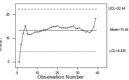
chart and R chart from the first risk (g=1) seem to be in state of statistical control, for the aluminum and plastic covariates as in Figure 1, 2, 3 and 4. On one hand, the wood covariate from the same data has one point observed to be above upper control bound as clearly shown in Figure 5. On the other hands, Figure 6, which associated with R chart, gives evidence of the presence of all the observation which are in state of statistical control. This results indicates that the tube wrapped on aluminum and plastic mandrels have along survival compared to the one wrapped on wooden mandrel. However, the results might be attributed to the second risk (g=2), which showed the tube wrapped on plastic mandrel have excellentcrashworthiness performance with respect to the chart and R chart as shown in Figure 9 and 10. on the
x
other hand Figures 7 and 11 show the chart for the aluminum and wood covariates. It can be seen that
x
some observations found to be below the lower bounds of control limit. In contrast from chart,
x
R chartgives an indication that the aluminum and wooed covariates are in the state of control as seen in Figure 8 and 12. Note that Figures 7, 8, 11, and 12 is not addressed here.
Fig. 1: The control chart for aluminum mandrel with internal diameter of 0 mm (First Risk).
x
Fig. 2: The control chart for aluminum mandrel with internal diameter of 0 mm (First Risk).
x
Fig. 3: The control chart for plastic mandrel with internal diameter of 0 mm (First Risk).
x
Fig. 5: The control chart for wood mandrel with internal diameter of 0 mm (First Risk).
x
Fig. 6: The control chart for wood mandrel with internal diameter of 0 mm (First Risk).
x
Fig. 9 The control chart for plastic mandrel with internal diameter of 0 mm (Second Risk).
x
For this data set (i.e. thick-walled mandrel). The chart obtained from the two types of failure, for the
x
aluminum, plastic and wood shifting below the control limit (LCL) which is indicate that to be out of control as seen clearly in Figure 13, 15, 17, 19, 21 and 23. On the other hand, the R chart obtained from the two type of failure, for the aluminum, plastic and wood seem to be in state of control as seen in Figure 14, 16, 18, 20, 22 and 24 respectively. Note that Figures 13, 14, 15, 16, 17, 18, 19, 20, 21, 22, 23 and 24 is not addressed here.
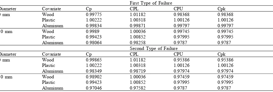
Table 1 show the estimates of the Cp, CPL, CPU and Cpk, obtained by the competing risks model, that
is, Cox’s model with Weibull distribution based on EM algorithm from two data sets of FCTD (0 mm and 10 mm). The value of Cpand Cpk for the first type of failure obtained from FCTD (di=0 and 10) are reasonably
closed to one for covariates wood, plastic and aluminum. Moreover, due the two type of failure for same data set, plastic mandrel provide the estimated of the Cp and Cpk values are greater than one, which is indicate that
the process is capable of producing items within desired limits.
6. Conclusion:
The parametric Cox’s proportional hazards regression model with Weibull distribution based on EM algorithm has been used successfully to investigate the causes of failure for statistical process control. The combination of the two data sets gives engineers the opportunity to perform analysis of more than one stress-type. Even though, from the analysis the first type of failure (stress) is significant, we have an insight of other causes that may can bute to the failure. The result obtained by proposed model for statistical process control technique in equations (1), (2), (3), (12), (13) based on equation (19) can be used effectively in the analysis of reliability data. Plastic mandrel shows that the process is under control but operating at an unacceptable level for covariates aluminum and wood. There is no evidence to indicate that the production of nonconforming units is operator controllable. It is quite clear to improve the energy absorption capability of woven roving composite tubes; they must be wrapped over a well design mandrel, such as the plastic one. Follow-up research should cover the application of these methods to simulation data.
Table 1: Comparison of the wood, plastic and aluminum with internal diameter 0 and 10 mm, obtained by PHW for Process Capability Index
First Type of Failure
Diameter Covariate Cp CPL CPU Cpk
0 mm Wood 0.99775 1.01182 0.98368 0.98368
Plastic 1.00222 1.00318 1.00126 1.00126
Aluminum 0.99834 0.99871 0.99797 0.99797
10 mm Wood 0.9989 1.00036 0.99745 0.99745
Plastic 0.99423 1.00852 0.97995 0.97995
Aluminum 0.98064 0.98258 0.9787 0.9787
Second Type of Failure
Diameter Covariate Cp CPL CPU Cpk
0 mm Wood 0.99865 1.01182 0.95386 0.95386
Plastic 1.00222 1.00318 1.00126 1.00126
Aluminum 0.98349 0.98719 0.97974 0.97974
10 mm Wood 0.98902 1.00036 0.97459 0.97459
Plastic 0.99423 1.00852 0.97995 0.97995
Aluminum 0.97046 0.97582 0.9787 0.9787
REFERENCE
Aly, A.A.E., S.C. Kochar and I.W. Mckeague, 1994. “Some Tests For Comparing. Cumulative Incidence Functions and Cause-Specific Hazard Rates.” American. S. A. J., 89: 994-999.
Besterfield. D.H., 1986 “Quality Control.” Second Edition. Prentice-Hall.
Chan, L.K., S.W. Cheng and F.A. Spiring, 1988. “A New Measure of Process Capability: Cpm.” J. Qual.
Technol., 20: 162-175.
Cheng, S.C., J.P. Fine and L.J. Wej, 1998. “Prediction of Cumulative Incidence Function Under the Proportional Hazards Model.” Biometrics, 54: 219-228.
Chou, Y., D.B. Owen and S.A. Borrego, 1990. “Lower Confidence Limits on Process Capability Indices.” Journal of Quality Technology, 22(3): 223-229.
Cox, D.R., 1972. “Regression Models and Life Tables (with discussion).” J R. Statist. Soc. 34: 187-220. Dhillon, B.S., 1985. “Quality Control, Reliability, and Engineering Design.” Marcel Dekker, INC. Duncan, A.J., 1974. “Quality Control and Industrial Statistics, 4th ed., Irwin, Homewood, III.
Grant, E.L. and R.S. Leavenworth, 1980. “Statistical Quality Control, 5th
ed., McGraw-Hill, New York. Gunter, B.H., 1989. “The Use and Abuse of Cpk.” Quality Progress, 22(4): 72-73.
Kalbfleisch, J.D. and J.F. Lawless, 1988. “Estimation of Reliability in Field-Performance Studies.” Technometrics, 30: 365-388.
Kane, V.E., 1986. “Process Capability Indices.” J. Qual. Technol., 18: 41-52. Lawless, J.F., 1983. “Statistical Methods In Reliability.” Technometrics, 25: 305-335.
Mahdi, E., 2003.“The influence of mandrel rigidity on the crushing behaviour of woven roving glass/epoxy wound laminated tubes.
AMPT, 2003.” Dublin, Ireland Montgomery, D.C. (1985) “Introduction to Statistical Quality Control.” John Wiley & Sons, New York, NY.
Nedumaran, G. and J.J. Pignatiello, 2001. “On Estimating Control Chart Limits.” J. Qual. Technol.,X 33(2): 206-212.
Owen, D.B. and T.A. Hau, 1977. “Tables of Confidence Limits on Tail area of the Normal Distribution.” Communications in Statistics, B6(3): 285-310.
Parlar, M. and G.O. Wesolowsky, 1999. “Specification Limits, Capability Indices, and Process Centering in Assembly Manufacture.” J. Qual. Technol., 31(3): 317-325.
Peto, R.R. and P. Lee, 1973. “Weibull Distributions for Continuous Carcinogensis Experiments.” Biometrics, 29: 457-470.
Pike, M.C., 1966. “A Method of Analysis of A Certain Class of Experiments In Carcinogensis”. Biometrics, 22: 142-161.
Rado, L.E., 1989. “Enhance Product Development by Using Capability Indexes.” Quality Progress, 22(4): 38-41.
Ryan, T.P., 1989. “Statistical Methods for Quality Improvement.” John Wiley & Sons, New York, NY. Spiring, F.A., 1991. “Cpm index.” Quality Process., 24: 57-61.
Stoumbos, Z.G., 2002. “Process Capability Indices: Overview and Extensions.” Journal of Nonliner Analysis: Real World Applications, 3: 191-210.
Stuart, M., E. Mullins and E. Drew, 1996 “Statistical Quality Control and Improvement.” European Journal of Operational Research, 88: 203-214.
Wadsworth, H.M., K.S. Stephens and A.B. Godfrey, 1986. “Modern Methods for Quality Control and Improvement.” John Wiley and Sons, New York.