The Geometry & Topology of 3 Manifold Thurston

(1)

William P. Thurston

The Geometry and Topology of Three-Manifolds

Electronic version 1.1 - March 2002 http://www.msri.org/publications/books/gt3m/

This is an electronic edition of the 1980 notes distributed by Princeton University. The text was typed in TEX by Sheila Newbery, who also scanned the figures. Typos have been corrected (and probably others introduced), but otherwise no attempt has been made to update the contents. Genevieve Walsh compiled the index.

Numbers on the right margin correspond to the original edition’s page numbers. Thurston’sThree-Dimensional Geometry and Topology, Vol. 1 (Princeton University Press, 1997) is a considerable expansion of the first few chapters of these notes. Later chapters have not yet appeared in book form.

(2)

(3)

Introduction

These notes (through p. 9.80) are based on my course at Princeton in 1978– 79. Large portions were written by Bill Floyd and Steve Kerckhoff. Chapter 7, by John Milnor, is based on a lecture he gave in my course; the ghostwriter was Steve Kerckhoff. The notes are projected to continue at least through the next academic year. The intent is to describe the very strong connection between geometry and low-dimensional topology in a way which will be useful and accessible (with some effort) to graduate students and mathematicians working in related fields, particularly 3-manifolds and Kleinian groups.

(4)

(5)

Geometry and three-manifolds

1.1 The theme I intend to develop is that topology and geometry, in dimensions up through 3, are very intricately related. Because of this relation, many questions which seem utterly hopeless from a purely topological point of view can be fruitfully studied. It is not totally unreasonable to hope that eventually all three-manifolds will be understood in a systematic way. In any case, the theory of geometry in three-manifolds promises to be very rich, bringing together many threads.

Before discussing geometry, I will indicate some topological constructions yielding diverse three-manifolds, which appear to be very tangled.

0. Start with the three sphereS3

, which may be easily visualized as R3

, together with one point at infinity.

1. Any knot (closed simple curve) or link (union of disjoint closed simple curves) may be removed. These examples can be made compact by removing the interior of a tubular neighborhood of the knot or link.

(10)

1. GEOMETRY AND THREE-MANIFOLDS

The complement of a knot can be very enigmatic, if you try to think about it from an intrinsic point of view. Papakyriakopoulos proved that a knot complement has fundamental groupZif and only if the knot is trivial. This may seem intuitively clear, but justification for this intuition is difficult. It is not known whether knots with homeomorphic complements are the same.

2. Cut out a tubular neighborhood of a knot or link, and glue it back in by a different identification. This is called Dehn surgery. There are many ways to do this, because the torus has many diffeomorphisms. The generator of the kernel of the inclusion map π1(T

2

) → π1 (solid torus) in the resulting three-manifold determines the three-manifold. The diffeomorphism can be chosen to make this generator an arbitrary primitive (indivisible non-zero) element of Z⊕_Z. It is well defined up to change in sign.

Every oriented three-manifold can be obtained by this construction (Lickorish) . It is difficult, in general, to tell much about the three-manifold resulting from this construction. When, for instance, is it simply connected? When is it irreducible? (Irreducible means every embedded two sphere bounds a ball).

Note that the homology of the three-manifold is a very insensitive invariant. The homology of a knot complement is the same as the homology of a circle, so when Dehn surgery is performed, the resulting manifold always has a cyclic first homology group. If generators forZ⊕_Z=π1(T

2

) are chosen so that (1,0) generates the homology of the complement and (0,1) is trivial then any Dehn surgery with invariant (1, n) yields a homology sphere. 3. Branched coverings. If L is a link, then any finite-sheeted covering space of S3

−L can be compactified in a canonical way by adding circles which cover L to give a closed manifold, M. M is called a 1.3 branched covering ofS3

overL. There is a canonical projectionp:M →S3

, which is a local diffeomorphism away fromp−1

(L). IfK ⊂S3

is a knot, the simplest branched coverings of S3

over K are then n-fold cyclic branched covers, which come from the covering spaces of S3

−K whose fundamental group is the kernel of the composition π1(S from K n times. If K is the trivial knot the cyclic branched covers are S3

. It seems intuitively obvious (but it is not known) that this is the only way S3

can be obtained as a cyclic branched covering of itself over a knot. Montesinos and Hilden (independently) showed that every oriented three-manifold is a branched cover of S3 with 3 sheets, branched over some knot. These branched coverings are not in general regular: there are no covering transformations.

The formation of irregular branched coverings is somehow a much more flexible construction than the formation of regular branched coverings. For instance, it is not hard to find many different ways in whichS3

(11)

5. Heegaard decompositions. Every three-manifold can be obtained from two handlebodies (of some genus) by gluing their boundaries together.

1.4 The set of possible gluing maps is large and complicated. It is hard to tell, given two gluing maps, whether or not they represent the same three-manifold (except when there are homological invariants to distinguish them).

6. Identifying faces of polyhedra. Suppose P1, . . . , Pk are polyhedra such that the number of faces withK sides is even, for each K.

Choose an arbitrary pattern of orientation-reversing identifications of pairs of two-faces. This yields a three-complex, which is an oriented manifold except near the vertices. (Around an edge, the link is automatically a circle.)

There is a classical criterion which says that such a complex is a manifold if and only if its Euler characteristic is zero. We leave this as an exercise.

In any case, however, we may simply remove a neighborhood of each bad vertex, to obtain a three-manifold with boundary.

The number of (at least not obviously homeomorphic) three-manifolds grows very quickly with the complexity of the description. Consider, for instance, different ways to obtain a three-manifold by gluing the faces of an octahedron. There are

8! 24_·

4!·3 4

= 8,505

possibilities. For an icosahedron, the figure is 38,661 billion. Because these polyhedra are symmetric, many gluing diagrams obviously yield homeomorphic results—but this reduces the figure by a factor of less than 120 for the icosahedron, for instance.

In two dimensions, the number of possible ways to glue sides of 2n-gon to obtain an oriented surface also grows rapidly with n: it is (2n)!/(2n

(12)

such a phenomenon takes place among three-manifolds; but how can we tell?

Example. _{Here is one of the simplest possible gluing diagrams for a}

three-manifold. Begin with two tetrahedra with edges labeled:

There is a unique way to glue the faces of one tetrahedron to the other so that arrows are matched. For instance, A is matched with A′_{. All the} _6−→ _{arrows are} identified and all the 6 6 −→ arrows are identified, so the resulting complex has 2 tetrahedra, 4 triangles, 2 edges and 1 vertex. Its Euler characteristic is +1, and (it follows that) a neighborhood of the vertex is the cone on a torus. Let M be the manifold obtained by removing the vertex.

(13)

1.6

Another view of the figure-eight knot

This knot is familiar from extension cords, as the most commonly occurring knot, after the trefoil knot

In order to see this homeomorphism we can draw a more suggestive picture of the figure-eight knot, arranged along the one-skeleton of a tetrahedron. The knot can be

(14)

spanned by a two-complex, with two edges, shown as arrows, and four two-cells, one for each face of the tetrahedron, in a more-or-less obvious way: 1.7

This pictures illustrates the typical way in which a two-cell is attached. Keeping in mind that the knot is not there, the cells are triangles with deleted vertices. The two complementary regions of the two-complex are the tetrahedra, with deleted vertices. We will return to this example later. For now, it serves to illustrate the need for a systematic way to compare and to recognize manifolds.

Note. _{Suggestive pictures can also be deceptive. A trefoil knot can similarly be}

(15)

From the picture, a cell-division of the complement is produced. In this case, however, the three-cells are not tetrahedra.

(16)

CHAPTER 2

Elliptic and hyperbolic geometry

There are three kinds of geometry which possess a notion of distance, and which look the same from any viewpoint with your head turned in any orientation: these are elliptic geometry (or spherical geometry), Euclidean or parabolic geometry, and hyperbolic or Lobachevskiian geometry. The underlying spaces of these three geome-tries are naturally Riemannian manifolds of constant sectional curvature +1, 0, and

−1, respectively.

Elliptic n-space is the n-sphere, with antipodal points identified. Topologically it is projective n-space, with geometry inherited from the sphere. The geometry of elliptic space is nicer than that of the sphere because of the elimination of identical, antipodal figures which always pop up in spherical geometry. Thus, any two points in elliptic space determine a unique line, for instance.

In the sphere, an object moving away from you appears smaller and smaller, until it reaches a distance of π/2. Then, it starts looking larger and larger and optically, it is in focus behind you. Finally, when it reaches a distance ofπ, it appears so large that it would seem to surround you entirely.

2.2

(17)

2. ELLIPTIC AND HYPERBOLIC GEOMETRY

distressing to live in elliptic space, since you would always be confronted with an im-age of yourself, turned inside out, upside down and filling out the entire background of your field of view. Euclidean space is familiar to all of us, since it very closely approximates the geometry of the space in which we live, up to moderate distances. Hyperbolic space is the least familiar to most people. Certain surfaces of revolution in R3 have constant curvature ₋1 and so give an idea of the local picture of the

hyperbolic plane. 2.3

The simplest of these is the pseudosphere, the surface of revolution generated by a tractrix. A tractrix is the track of a box of stones which starts at (0,1) and is dragged by a team of oxen walking along thex-axis and pulling the box by a chain of unit length. Equivalently, this curve is determined up to translation by the property that its tangent lines meet thex-axis a unit distance from the point of tangency. The pseudosphere is not complete, however—it has an edge, beyond which it cannot be extended. Hilbert proved the remarkable theorem that no complete C2 _{surface with}

curvature ₋1 can exist in _R3_{. In spite of this, convincing physical models can be}

constructed.

We must therefore resort to distorted pictures of hyperbolic space. Just as it is convenient to have different maps of the earth for understanding various aspects of its geometry: for seeing shapes, for comparing areas, for plotting geodesics in navigation; so it is useful to have several maps of hyperbolic space at our disposal.

2.1. The Poincar´e disk model.

(18)

2.2. THE SOUTHERN HEMISPHERE.

the extended sense, to include the limiting case of a line or plane. This model is conformally correct, that is, hyperbolic angles agree with Euclidean angles, but distances are greatly distorted. Hyperbolic arc length√ds2 _{is given by the formula} _2.4

ds2 = 1 1₋r2

2

dx2,

where √dx2 _{is Euclidean arc length and} _r _{is distance from the origin. Thus, the}

Euclidean image of a hyperbolic object, as it moves away from the origin, shrinks in size roughly in proportion to the Euclidean distance from ∂Dn _{(when this distance} is small). The object never actually arrives at ∂Dn_{, if it moves with a bounded} hyperbolic velocity.

The sphere ∂Dn _{is called the} _{sphere at infinity}_{. It is not actually in hyperbolic} space, but it can be given an interpretation purely in terms of hyperbolic geometry, as follows. Choose any base point p0 in Hn_{. Consider any geodesic ray} _R_{, as seen} from p0. R traces out a segment of a great circle in the visual sphere at p0 (since

p0 and R determine a two-plane). This visual segment converges to a point in the visual sphere. If we translateHn _{so that}_p0 _{is at the origin of the Poincar´e disk} _2.5

model, we see that the points in the visual sphere correspond precisely to points in the sphere at infinity, and that the end of a ray in this visual sphere corresponds to its Euclidean endpoint in the Poincar´e disk model.

2.2. The southern hemisphere.

The Poincar´e disk Dn_⊂_Rn _{is contained in the Poincar´e disk} _Dn+1 _⊂_Rn+1_{, as a}

(19)

Stereographic projection (Euclidean) from the north pole of ∂Dn+1 _{sends the}

Poincar´e disk Dn _{to the southern hemisphere of} _Dn+1_.

Thus hyperbolic lines in the Poincar´e disk go to circles on Sn _{orthogonal to the} equator Sn−1_.

There is a more natural construction for this map, using only hyperbolic geometry. For each point p inHn

⊂Hn+1_{, consider the hyperbolic ray perpendicular to} _Hn _at

p, and downward normal. This ray converges to a point on the sphere at infinity, 2.6

which is the same as the Euclidean stereographic image of p.

2.3. The upper half-space model.

This is closely related to the previous two, but it is often more convenient for computation or for constructing pictures. To obtain it, rotate the sphere Sn _in Rn+1 _{so that the southern hemisphere lies in the half-space} _x

(20)

2.4. THE PROJECTIVE MODEL.

stereographic projection from the top of Sn _{(which is now on the equator) sends the} southern hemisphere to the upper half-spacexn >0 in Rn+1. 2.7

A hyperbolic line, in the upper half-space, is a circle perpendicular to the bounding plane _Rn−1 _⊂

Rn. The hyperbolic metric is ds2 _{= (1}_/x_n)2_dx2_{. Thus, the Euclidean}

image of a hyperbolic object moving toward _Rn−1 _{has size precisely proportional to}

the Euclidean distance from Rn−1_.

2.4. The projective model.

This is obtained by Euclidean orthogonal projection of the southern hemisphere of Sn _{back to the disk} _Dn_{. Hyperbolic lines become Euclidean line segments. This} model is useful for understanding incidence in a configuration of lines and planes. Unlike the previous three models, it fails to be conformal, so that angles and shapes are distorted.

It is better to regard this projective model to be contained not in Euclidean space, but in projective space. The projective model is very natural from a point of 2.8

(21)

as the interior of a disk in his visual sphere. As he moves farther up, this visual disk shrinks; as he moves down, it expands; but (unlike in Euclidean space), the visual radius of this disk is always strictly less than π/2. A line on H2 _{appears visually}

straight.

It is possible to give an intrinsic meaning within hyperbolic geometry for the points outside the sphere at infinity in the projective model. For instance, in the two-dimensional projective model, any two lines meet somewhere. The conventional sense of meeting means to meet inside the sphere at infinity (at a finite point). If the two lines converge in the visual circle, this means that they meet on the circle at infinity, and they are calledparallels. Otherwise, the two lines are calledultraparallels; they have a unique common perpendicular L and they meet in some point x in the M¨obius band outside the circle at infinity. Any other line perpendicular to L passes through x, and any line through x is perpendicular to L. 2.9

To prove this, consider hyperbolic two-space as a plane P _⊂ H3_{. Construct}

the plane Q through L perpendicular to P. Let U be an observer in H3_{. Drop a}

(22)

2.4. THE PROJECTIVE MODEL.

2.8a

Evenly spaced lines. The region inside the circle is a plane, with a base line and a family of its perpendiculars, spaced at a distance of ._{051 fundamental units, as measured along the base}

line shown in perspective in hyperbolic 3-space (or in the projective model). The lines have been extended to their imaginary meeting point beyond the horizon. U_{, the observer, is directly above}

theX _{(which is} ._{881 fundamental units away from the base line). To see the view from different}

heights, use the following table (which assumes that the Euclidean diameter of the circle in your printout is about 5.25 inches or 13.3cm):

To see the view of hold the picture a

U _{at a height of} _{distance of}

2 units 11′′_{( 28 cm)}

3 units 27′′_{( 69 cm)}

4 units 6′ _{(191 cm)}

To see the view of hold the picture a

U _{at a height of} _{distance of}

5 units 17′ _{(519 cm)}

10 units 2523′ _{(771 m )}

(23)

to L, the plane determined by U and K is perpendicular to Q, hence contains M; hence the visual line determined by K in the visual sphere of U passes through the visual point determined by K. The converse is similar. 2.10

This gives a one-to-one correspondence between the set of points x outside the sphere at infinity, and (in general) the set of hyperplanes L in Hn_. _L _corresponds to the common intersection point of all its perpendiculars. Similarly, there is a correspondence between points inHn _{and hyperplanes outside the sphere at infinity:} a pointpcorresponds to the union of all points determined by hyperplanes throughp.

2.5. The sphere of imaginary radius.

A sphere in Euclidean space with radius r has constant curvature 1/r2_{. Thus,}

hyperbolic space should be a sphere of radiusi. To give this a reasonable interpreta-tion, we use an indefinite metricdx2 ₌_dx2

1+· · ·+dx2n−dx2n+1 inRn+1. The sphere

of radius i about the origin in this metric is the hyperboloid

(24)

2.6. TRIGONOMETRY.

2.11

The metric dx2 _{restricted to this hyperboloid is positive definite, and it is not}

hard to check that it has constant curvature₋1. Any plane through the origin isdx2

-orthogonal to the hyperboloid, so it follows from elementary Riemannian geometry that it meets the hyperboloid in a geodesic. The projective model for hyperbolic space is reconstructed by projection of the hyperboloid from the origin to a hyperplane in Rn. Conversely, the quadratic form x2

1 +· · ·+x2n−x2n+1 can be reconstructed from

the projective model. To do this, note that there is a unique quadratic equation of the form

n X

i,j=1

aijxixj = 1

defining the sphere at infinity in the projective model. Homogenization of this equa-tion gives a quadratic form of type (n,1) in Rn+1_{, as desired. Any isometry of the}

quadratic form x2

1 +· · ·+x2n −x2n+1 induces an isometry of the hyperboloid, and

hence any projective transformation of Pn _{that preserves the sphere at infinity} in-duces an isometry of hyperbolic space. This contrasts with the situation in Euclidean geometry, where there are many projective self-homeomorphisms: the affine transfor-mations. In particular, hyperbolic space has no similarity transformations except isometries. This is true also for elliptic space. This means that there is a well-defined unit of measurement of distances in hyperbolic geometry. We shall later see how this is related to three-dimensional topology, giving a measure of the “size” of manifolds. 2.12

2.6. Trigonometry.

(25)

space as one sheet of the “sphere” of radius i with respect to the quadratic form

Q(X) = X₁2 +_{· · ·}+X_n2₋X_n2₊₁

in _Rn+1_{. The set}

Rn+1, equipped with this quadratic form and the associated inner product

is calledEn,1_{. First we will describe the geodesics on level sets}_S

r={X :Q(X) =r2} of Q. Suppose thatXt is such a geodesic, with speed

s=

Since any geodesic must lie in a two-dimensional subspace, ¨Xt must be a linear combination of Xt and ˙Xt, and we have

This differential equation, together with the initial conditions 2.13 X0_·X0 =r2, X0˙ _·X0˙ =s2, X0_·X0˙ = 0,

where _kX_k=√X_·X is positive real or positive imaginary. Note that

c(X, Y) = c(λX, µY),

whereλandµare positive constants, thatc(₋X, Y) =₋c(X, Y), and thatc(X, X) = 1. In Euclidean space En+1_,_c₍_{X, Y}_{) is the cosine of the angle between}_X _and _Y_{. In} En,1 _{there are several cases.}

We identify vectors on the positive sheet ofSi (Xn+1 >0) with hyperbolic space.

(26)

2.6. TRIGONOMETRY.

We will use the notation Y⊥ _{to denote this hyperplane,} _{with the normal orientation}

determined by Y. (We have seen this correspondence before, in 2.4.) 2.6.2. IfX and Y _∈Hn_{, then} _c₍_{X, Y}_{) = cosh}_d₍_{X, Y}₎_, where d(X, Y) denotes the hyperbolic distance betweenX and Y.

To prove this formula, joinX toY by a geodesicXt of unit speed. From 2.6.1 we 2.14 have

¨

Xt=Xt, Xt·X0˙ = 0,

so we get c( ¨Xt, Xt) =c(Xt, Xt), c( ˙X0, X0) = 0, c(X, X0) = 1; thusc(X, Xt) = cosht. When t=d(X, Y), then Xt=Y, giving 2.6.2.

IfX⊥ _and _Y⊥ _{are distinct hyperplanes, then} 2.6.3.

X⊥ _and _Y⊥ _intersect

⇐⇒ Qis positive definite on the subspace _hX, Y_i spanned by X and Y ⇐⇒ c(X, Y)2 <1

=_⇒c(X, Y) = cos∠(X, Y) = ₋cos∠(X⊥, Y⊥).

To see this, note thatX and Y intersect in Hn

⇐⇒ Q restricted toX⊥_∩_Y⊥ _is indefinite of type (n₋2,1) _⇐⇒ Q restricted to_hX, Y_i is positive definite. (_hX, Y_i

is the normal subspace to the (n₋2) plane X⊥_∩_Y⊥_). _2.15 There is a general elementary formula for the area of a parallelogram of sidesX

and Y with respect to an inner product:

area =pX_·X Y _·Y ₋(X_·Y)2 ₌_k_X_{k · k}_Y_{k ·}p₁₋_c₍_{X, Y}₎2_.

This area is positive real if X and Y span a positive definite subspace, and pos-itive imaginary if the subspace has type (1,1). This shows, finally, that X⊥ _and

Y⊥ _intersect _⇐⇒ _c₍_{X, Y}₎2 _< _{1. The formula for} _c₍_{X, Y}_{) comes from ordinary}

(27)

2.6.4.

X⊥ _and _Y⊥ _{have a common perpendicular} _⇐⇒ _Q _{has type (1}_,_{1) on} _h_{X, Y}_i

⇐⇒ c(X, Y)2 >1

=_⇒c(X, Y) = _±cosh d(X⊥_{, Y}⊥₎

.

The sign is positive if the normal orientations of the common perpendiculars coincide, and negative otherwise.

2.16

The proof is similar to 2.6.2. We may assume X and Y have unit length. Since

hX, Y_i intersects Hn _{as the common perpendicular to} _X⊥ _and _Y⊥_, _Q _{restricted to}

hX, Y_i has type (1,1). Replace X by ₋X if necessary so that X and Y lie in the same component ofS1_∩hX, Y_i. JoinX toY by a geodesicXtof speedi. From 2.6.1,

¨

Xt = Xt. There is a dual geodesic Zt of unit speed, satisfying Zt·Xt = 0, joining

X⊥ _to _Y⊥ _{along their common perpendicular, so one may deduce that}

c,(X, Y) = _±d(X,Y_i ) =_±d(X⊥, Y⊥).

There is a limiting case, intermediate between 2.6.3 and 2.6.4:

2.6.5. X⊥ _and _Y⊥ _{are parallel}

⇐⇒ Q restricted to_hX, Y_i is degenerate

⇐⇒ c(X, Y)2 = 1.

(28)

2.6. TRIGONOMETRY. There is one more case in which to interpretc(X, Y):

2.6.6. If X is a point inHn _and _Y⊥ _{a hyperplane, then}

c(X, Y) = sinh d(X, Y ⊥₎

i ,

where d(X, Y⊥_{) is the} _oriented _distance. _2.17

The proof is left to the untiring reader.

With our dictionary now complete, it is easy to derive hyperbolic trigonometric formulae from linear algebra. To solve triangles, note that the edges of a triangle with vertices u, v and w in H2 _are _U⊥_,_V⊥ _and _W⊥_{, where} _U _{is a vector orthogonal} to v and w, etc. To find the angles of a triangle from the lengths, one can find three vectors u,v, and wwith the appropriate inner products, find a dual basis, and calculate the angles from the inner products of the dual basis. Here is the general formula. We consider triangles in the projective model, with vertices inside or outside the sphere at infinity. Choose vectorsv1,v2 andv3 of lengthior 1 representing these

points. Let ǫi = vi ·vi, ǫij = √ǫiǫj and cij = c(vi, vj). Then the matrix of inner products of the vi is

C = 



ǫ1 ǫ12c12 ǫ13c13 ǫ12c12 ǫ2 ǫ23c23 ǫ13c13 ǫ23c23 ǫ3



.

The matrix of inner products of the dual basis _{v1_{, v}2_{, v}3_} _is _C−1_{. For our} pur-2.18

(29)

where it is easy to deduce the sign

ǫ= _√ −ǫ12ǫ3

−ǫ2ǫ3√₋ǫ1ǫ3

(30)

2.6. TRIGONOMETRY.

2.6.10. coshC = coshαcoshβ+ coshγ sinhαsinhβ .

(See also 2.6.18.) Such hexagons are useful in the study of hyperbolic structures on surfaces. Similar formulas can be obtained for pentagons with four right angles, or quadrilaterals with two adjacent right angles:

2.20

(31)

γ α

β C

2.6.11. coshC= cosαcosβ+ 1

sinαsinβ ,

and in particular

2.6.12. coshC = 1

sinα.

These formulas for a right triangle are worth mentioning separately, since they are

(32)

2.6. TRIGONOMETRY.

From the formula for cosγ we obtain the hyperbolic Pythagorean theorem:

2.6.13. coshC = coshAcoshB.

Also,

2.6.14. coshA= cosα

sinβ.

(Note that (cosα)/(sinβ) = 1 in a Euclidean right triangle.) By substituting (coshC)

(coshA) for coshB in the formula 2.6.9 for cosα, one finds:

2.6.15. In a right triangle, sinα = sinhA sinhC.

This follows from the general law of sines,

2.6.16. In any triangle,sinhA sinα =

sinhB

sinβ =

sinhC

sinγ .

2.22

(33)

one has

2.6.17. sinhAsinhB = coshD.

It follows that in any all right hexagon,

there is a law of sines:

2.6.18. sinhA

sinhα =

sinhB

sinhβ =

sinhC

(34)

CHAPTER 3

Geometric structures on manifolds

A manifold is a topological space which is locally modelled onRn_{. The notion of}

what it means to be locally modelled on Rn _{can be made definite in many different}

ways, yielding many different sorts of manifolds. In general, to define a kind of manifold, we need to define a set G of gluing maps which are to be permitted for piecing the manifold together out of chunks of Rn_{. Such a manifold is called a} _G

-manifold. G should satisfy some obvious properties which make it a pseudogroup of local homeomorphisms between open sets of Rn_:

(i) The restriction of an elementg ∈G _{to any open set in its domain is also in} G.

(ii) The composition g1 ◦g2 of two elements of G, when defined, is in G.

(iii) The inverse of an element of G is in G.

(iv) The property of being in Gis local, so that if U =S_αUα and if g is a local

homeomorphismg :U →V whose restriction to eachUα is inG, theng ∈G.

It is convenient also to permit G to be a pseudogroup acting on any manifold, although, as long asGis transitive, this doesn’t give any new types of manifolds. See Haefliger, in Springer Lecture Notes #197, for a discussion.

A group G acting on a manifold X determines a pseudogroup which consists of restrictions of elements ofGto open sets inX. A (G, X)-manifold means a manifold 3.2

glued together using this pseudogroup of restrictions of elements ofG.

Examples. _If G _{is the pseudogroup of local} _Cr _{diffeomorphisms of} _Rn_{, then}

a G-manifold is a Cr_{-manifold, or more loosely, a differentiable manifold (provided}

r≥1).

If G is the pseudogroup of local piecewise-linear homeomorphisms, then a G -manifold is a PL--manifold. If G is the group of affine transformations of Rn_{, then a}

(G,Rn_{)-manifold is called an} _affine _{manifold. For instance, given a constant} _{λ >} ₁

(35)

3. GEOMETRIC STRUCTURES ON MANIFOLDS

3.3

Here is another method, due to John Smillie, for constructing affine structures on T2 _{from any quadrilateral} _Q _{in the plane. Identify the opposite edges of} _Q _by

the orientation-preserving similarities which carry one to the other. Since similarities preserve angles, the sum of the angles about the vertex in the resulting complex is 2π, so it has an affine structure. We shall see later how such structures on T2 _are

intimately connected with questions concerning Dehn surgery in three-manifolds.

The literature about affine manifolds is interesting. Milnor showed that the only closed two-dimensional affine manifolds are tori and Klein bottles. The main unsolved question about affine manifolds is whether in general an affine manifold has Euler characteristic zero.

If G is the group of isometries of Euclidean space En_{, then a (G, E}n_)-manifold

is called a Euclidean manifold, or often a flat manifold. Bieberbach proved that a Euclidean manifold is finitely covered by a torus. Furthermore, a Euclidean structure automatically gives an affine structure, and Bieberbach proved that closed Euclidean manifolds with the same fundamental group are equivalent as affine manifolds. If G is the group O(n+ 1) acting on elliptic space Pn _{(or on} _Sn_{), then we obtain} _elliptic

manifolds.

Conjecture. _{Every three-manifold with finite fundamental group has an elliptic}

(36)

3.1. A HYPERBOLIC STRUCTURE ON THE FIGURE-EIGHT KNOT COMPLEMENT.

This conjecture is a stronger version of the Poincar´e conjecture; we shall see the logic shortly. All known three-manifolds with finite fundamental group certainly have

elliptic structures. 3.4

As a final example (for the present), whenG is the group of isometries of hyper-bolic space Hn_{, then a (G, H}n_{)-manifold is a} _hyperbolic _{manifold. For instance, any}

surface of negative Euler characteristic has a hyperbolic structure. The surface of genus two is an illustrative example.

Topologically, this surface is obtained by identifying the sides of an octagon, in the pattern above, for instance. An example of a hyperbolic structure on the surface is obtained form any hyperbolic octagon whose opposite edges have equal lengths and whose angle sum is 2π, by identifying in the same pattern. There is a regular

octagon with angles π/4, for instance. 3.5

3.6

3.1. A hyperbolic structure on the figure-eight knot complement.

Consider a regular tetrahedron in Euclidean space, inscribed in the unit sphere, so that its vertices are on the sphere. Now interpret this tetrahedron to lie in the projective model for hyperbolic space, so that it determines an ideal hyperbolic sim-plex: combinatorially, a simplex with its vertices deleted. The dihedral angles of the hyperbolic simplex are 60◦_{. This may be seen by extending its faces to the sphere at}

infinity, which they meet in four circles which meet each other in 60◦ _angles.

By considering the Poincar´e disk model, one sees immediately that the angle made by two planes is the same as the angle of their bounding circles on the sphere at infinity.

Take two copies of this ideal simplex, and glue the faces together, in the pattern described in Chapter 1, using Euclidean isometries, which are also (in this case) hyperbolic isometries, to identify faces. This gives a hyperbolic structure to the

(37)

A regular octagon with angles π/4,

whose sides can be identified to give a surface of genus 2.

A tetrahedron inscribed in the unit sphere, top view.

(38)

3.2. A HYPERBOLIC MANIFOLD WITH GEODESIC BOUNDARY.

figure-eight knot is isomorphic to a subgroup of index 12 in PSL2(Z[ω]), where ω is

a primitive cube root of unity.

3.2. A hyperbolic manifold with geodesic boundary.

Here is another manifold which is obtained from two tetrahedra. First glue the two tetrahedra along one face; then glue the remaining faces according to this diagram:

3.8

In the diagram, one vertex has been removed so that the polyhedron can be flattened out in the plane. The resulting complex has only one edge and one vertex. The manifoldM obtained by removing a neighborhood of the vertex is oriented with boundary a surface of genus 2.

Consider now a one-parameter family of regular tetrahedra in the projective model for hyperbolic space centered at the origin in Euclidean space, beginning with the tetrahedron whose vertices are on the sphere at infinity, and expanding until the edges are all tangent to the sphere at infinity. The dihedral angles go from 60◦ _{to 0}◦_,

so somewhere in between, there is a tetrahedron with 30◦ _{dihedral angles. Truncate}

this simplex along each planev⊥_{, where}_v_{is a vertex (outside the unit ball), to obtain}

(39)

3.9

Two copies glued together give a hyperbolic structure forM, where the boundary of M (which comes from the triangular faces of the stunted simplices) is totally geo-desic. A closed hyperbolic three-manifold can be obtained by doubling this example, i.e., taking two copies of M and gluing them together by the “identity” map on the boundary.

3.3. The Whitehead link complement.

The Whitehead link may be spanned by a two-complex which cuts the complement into an octahedron, with vertices deleted:

The one-cells are the three arrows, and the attaching maps for the two-cells are indicated by the dotted lines. The three-cell is an octahedron (with vertices deleted), 3.10

(40)

3.4. THE BORROMEAN RINGS COMPLEMENT.

A hyperbolic structure may be obtained from a Euclidean regular octahedron in-scribed in the unit sphere. Interpreted as lying in the projective model for hyperbolic space, this octahedron is an ideal octahedron with all dihedral angles 90◦_.

3.11

Gluing it in the indicated pattern, again using Euclidean isometries between the faces (which happen to be hyperbolic isometries as well) gives a hyperbolic structure for the complement of the Whitehead link.

3.4. The Borromean rings complement.

(41)

Here is the corresponding gluing pattern of two octahedra. Faces are glued to their corresponding faces with 120◦ _{rotations, alternating in directions like gears.}

3.12

3.5. The developing map.

Let X be any real analytic manifold, and G a group of real analytic diffeomor-phisms of X. Then an element of G is completely determined by its restriction to any open set of X.

Suppose that M is any (G, X)-manifold. Let U1, U2, . . . be coordinate charts for

M, with mapsφi :Ui →X and transition functions γij satisfying

γij ◦φi =φj.

In general the γij’s are local G-diffeomorphisms ofX defined on φi(Ui∩Uj) so they

are determined by locally constant maps, also denoted γij, of Ui∩Uj into G.

Consider now an analytic continuation of φ1 along a path α in M beginning

(42)

3.5. THE DEVELOPING MAP.

continuation of φ1 along α is of the form γ ◦φi, where γ ∈ G. Hence, φ1 can be

analytically continued along every path in M. It follows immediately that there is a global analytic continuation of φ1 defined on the universal cover of M. (Use the

definition of the universal cover as a quotient space of the paths in M.) This map,

D: ˜M →X,

is called the developing map. D is a local (G, X)-homeomorphism (i.e., it is an im-mersion inducing the (G, X)-structure on ˜M.) Dis clearly unique up to composition 3.13

with elements of G.

Although G acts transitively onX in the cases of primary interest, this condition is not necessary for the definition of D. For example, if G is the trivial group and X is closed then closed (G, X)-manifolds are precisely the finite-sheeted covers of X, and D is the covering projection.

From this uniqueness property of D, we have in particular that for any covering transformationTα of ˜M over M, there is some (unique) element gα ∈Gsuch that

D◦Tα =gα◦D.

Since D◦Tα◦Tβ =gα◦D◦Tβ =gα◦gβ◦D it follows that the correspondence

H :α7→gα

is a homomorphism, called the holonomy of M.

In general, the holonomy of M need not determine the (G, X)-structure on M, but there is an important special case in which it does.

Definition. _M _{is a} _complete _{(G, X)-manifold if} _D _{: ˜}_M _→_X _{is a covering map.}

(In particular, if X is simply-connected, this means D is a homeomorphism.)

IfX is similarly connected, then any complete (G, X)-manifoldM may easily be reconstructed from the image Γ =H(π1(M)) of the holonomy, as the quotient space

X/Γ.

Here is a useful sufficient condition for completeness.

Proposition _3.6. _Let _G _{be a group of analytic diffeomorphisms acting}

transi-tively on a manifold X, such that for any x ∈ X, the isotropy group Gx of x is compact. Then every closed (G, X)-manifold M is complete.

Proof. _Let_Q_{be any positive definite on the tangent space}_T_x_{(X) of} _X _{at some}

point x. Average the set of transforms g(Q), g ∈Gx, using Haar measure, to obtain

a quadratic form onTx(X) which is invariant under Gx. Define a Riemannian metric 3.14

(ds2₎

y = g(Q) on X, where g ∈ G is any element taking x to y. This definition

(43)

Therefore, this metric pieces together to give a Riemannian metric on any (G, X )-manifold, which is invariant under any (G, X)- map.

IfM is any closed (G, X)-manifold, then there is some ǫ >0 such that the ǫ-ball in the Riemannian metric on M is always convex and contractible. If x is any point in X, then D−1_(B

ǫ/2(x)) must be a union of homeomorphic copies of Bǫ/2(x) in ˜M.

D evenly coversX, so it is a covering projection, and M is complete.

For example, any closed elliptic three-manifold has universal cover S3_{, so any}

simply-connected elliptic manifold is S3_{. Every closed hyperbolic manifold or}

Eu-clidean manifold has universal cover hyperbolic three-space or EuEu-clidean space. Such

manifolds are consequently determined by their holonomy. 3.15

3.16

Even for G and X as in proposition 3.6, the question of whether or not a non-compact (G, X)-manifold M is complete can be much more subtle. For example, consider the thrice-punctured sphere, which is obtained by gluing together two tri-angles minus vertices in this pattern:

A hyperbolic structure can be obtained by gluing two ideal triangles (with all vertices on the circle at infinity) in this pattern. Each side of such a triangle is isometric to the real line, so a gluing map between two sides may be modified by an arbitrary translation; thus, we have a family of hyperbolic structures in the thrice-punctured sphere parametrized by R3_{. (These structures need not be, and are not, all distinct.)}

Exactly one parameter value yields a complete hyperbolic structure, as we shall see presently.

Meanwhile, we collect some useful conditions for completeness of a (G, X )-struc-ture with (G, X) as in 3.6. For convenience, we fix some natural metrics on (G, X)- 3.17

structures. Labelled 3.7.p to avoid

multiple labels

Proposition _3.7. _With _{(G, X}₎ _{as above, a} _{(G, X}₎_-manifold _M _{is complete if}

and only if any of the following equivalent conditions is satisfied.

(a) M is complete as a metric space.

(44)

3.5. THE DEVELOPING MAP.

3.15

(45)

(c) For every k >0, all closed k-balls are compact.

(d) There is a family {St};t ∈ R, of compact sets which exhaust M, such that

St+a contains a neighborhood of radius a about St.

Proof. _{Suppose that} _M _{is metrically complete. Then ˜}_M _{is also metrically}

com-plete. We will show that the developing map D : ˜M → X is a covering map by proving that any path αt inX can be lifted to ˜M. In fact, let T ⊂[0,1] be a

maxi-mal connected set for which there is a lifting. SinceD is a local homeomorphism, T is open, and because ˜M is metrically complete, T is closed: hence, α can be lifted, soM is complete.

It is an elementary exercise to see that (b) ⇐⇒ (c) ⇐⇒ (d) =⇒ (a). For any point x0 ∈ X˜ there is some ǫ such that the ball Bǫ(x) is compact; this ǫ works for

allx∈X˜ since the group ˜Gof (G, X)-diffeomorphisms of ˜X is transitive. Therefore X satisfies (a), (b), (c) and (d). Finally if M is a complete (G, X)-manifold, it is

covered by ˜X, so it satisfies (b). The proposition follows.

3.18

3.8. Horospheres.

(46)

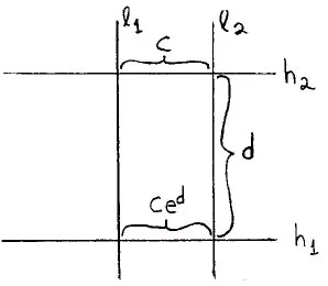
3.8. HOROSPHERES.

Concentric horocycles and orthogonal lines.

3.19

Translation along a line through X permutes the horospheres centered at X. Thus, all horospheres are congruent. The convex region bounded by a horosphere is ahoroball. For another view of a horosphere, consider the upper half-space model. In this case, hyperbolic lines through the point at infinity are Euclidean lines orthogonal to the plane bounding upper half-space. A horosphere about this point is a horizontal Euclidean plane. From this picture one easily sees that a horosphere inHn_{is isometric}

to Euclidean spaceEn−1_{. One also sees that the group of hyperbolic isometries fixing}

the point at infinity in the upper half-space model acts as the group of similarities of the bounding Euclidean plane. One can see this action internally as follows. Let X be any point at infinity in hyperbolic space, andhany horosphere centered at X. An isometry g of hyperbolic space fixing X takes h to a concentric horosphere h′_.

Project h′ _{back to} _h _{along the family of parallel lines through} _{X. The composition}

of these two maps is a similarity ofh.

Consider two directed lines l1 and l2 emanating from the point at infinity in the

upper half-space model. Recall that the hyperbolic metric is ds2 _{= (1/x}2

n)dx2. This

means that the hyperbolic distance betweenl1 and l2 along a horosphere is inversely

proportional to the Euclidean distance above the bounding plane. The hyperbolic distance between pointsX1 andX2 onl1 at heights ofh1 andh2 is|log(h2)−log(h1)|.

It follows that for any two concentric horospheres h1 and h2 which are a distance d

(47)

Figure 1. _{Horocycles and lines in the upper half-plane}

between l1 and l2 measured along h1 to their distance measured along h2 is exp(d).

3.9. Hyperbolic surfaces obtained from ideal triangles.

Consider an oriented surfaceS obtained by gluing ideal triangles with all vertices at infinity, in some pattern. Exercise: all such triangles are congruent. (Hint: you can derive this from the fact that a finite triangle is determined by its angles—see 2.6.8. Let the vertices pass to infinity, one at a time.)

Let K be the complex obtained by including the ideal vertices. Associated with each ideal vertex v of K, there is an invariant d(v), defined as follows. Let h be a horocycle in one of the ideal triangles, centered about a vertex which is glued to v and “near” this vertex. Extend h as a horocycle in S counter clockwise about v. It meets each successive ideal triangle as a horocycle orthogonal to two of the sides, until finally it re-enters the original triangle as a horocycle h′ _{concentric with} _{h, at a}

distance ±d(v) from h. The sign is chosen to be positive if and only if the horoball

(48)

3.9. HYPERBOLIC SURFACES OBTAINED FROM IDEAL TRIANGLES.

The surface S is complete if and only if all invariants d(v) are 0. Suppose, for instance, that some invariant d(v) < 0. Continuing h further round v; the length of each successive circuit around v is reduced by a constant factor <1, so the total length of h after an infinite number of circuits is bounded. A sequence of points evenly spaced along h is a non-convergent Cauchy sequence.

If all invariants d(v) = 0, on the other hand, one can remove horoball neighbor-hoods of each vertex inK to obtain a compact subsurface S0. Let St be the surface

obtained by removing smaller horoball neighborhoods bounded by horocycles a dis-tance of t from the original ones. The surfaces St satisfy the hypotheses of 3.7(d)

1—hence S is complete.

3.22

For any hyperbolic manifoldM, let ¯M be the metric completion ofM. In general, ¯

(49)

one boundary component of length|d(v)| for each vertex v of K such thatd(v)6= 0. ¯

Sis obtained by adjoining one limit point for each horocycle which “spirals toward” a vertex v inK. The most convincing way to understand ¯S is by studying the picture:

3.10. Hyperbolic manifolds obtained by gluing ideal polyhedra.

Consider now the more general case of a hyperbolic manifold M obtained by gluing together the faces of polyhedra in Hn _{with some vertices at infinity. Let} _K _3.23

be the complex obtained by including the ideal vertices. The link of an ideal vertex v is (by definition) the set L(v) of all rays through that vertex. From 3.7 it follows that the link of each vertex has a canonical (similarities of En−1_, _En−1 _{) structure,}

or similarity structure for short. An extension of the analysis in 3.9 easily shows that M is complete if and only if the similarity structure on each link of an ideal vertex is actually a Euclidean structure, or equivalently, if and only if the holonomy of these similarity structures consists of isometries. We shall be concerned mainly with dimension n = 3. It is easy to see from the Gauss-Bonnet theorem that any similarity two-manifold has Euler characteristic zero. (Its tangent bundle has a flat orthogonal connection). Hence, if M is oriented, each link L(v) of an ideal vertex is topologically a torus. If L(v) is not Euclidean, then for some α ∈ π1L(v), the

holonomyH(α) is a contraction, so it has a unique fixed pointx0. Any other element

β ∈ π1(L(v)) must also fix x0, since β commutes with α. Translating x0 to 0, we

see that the similarity two-manifoldL(v) must be a (C∗_,C₋_{0)-manifold where}C∗ _is

(50)

3.10. HYPERBOLIC MANIFOLDS OBTAINED BY GLUING IDEAL POLYHEDRA.

is automatically complete (by 3.6), and it is also modelled on

( ˜C∗_,_C^₋_0),

or, by taking logs, on (C,C). Here the first C is an additive group and the second

C _{is a space. Conversely, by taking exp, any (}C_,C_{) structure gives a similarity}

structure. (C,C) structures on closed oriented manifolds are easy to describe, being determined by their holonomy, which is generated by an arbitrary pair (z1, z2) of 3.24

complex numbers which are linearly independent over R.

(51)

CHAPTER 4

Hyperbolic Dehn surgery

A hyperbolic structure for the complement of the figure-eight knot was con-structed in 3.1. This structure was in fact chosen to be complete. The reader may wish to verify this by constructing a horospherical realization of the torus which is the link of the ideal vertex. Similarly, the hyperbolic structure for the Whitehead link complement and the Borromean rings complement constructed in 3.3 and 3.4 are complete.

There is actually a good deal of freedom in the construction of hyperbolic struc-tures for such manifolds, although most of the resulting strucstruc-tures are not complete. We shall first analyze the figure-eight knot complement. To do this, we need an understanding of the possible shapes of ideal tetrahedra.

4.1. Ideal tetrahedra in H3_.

The link L(v) of an ideal vertex v of an oriented ideal tetrahedron T (which by definition is the set of rays in the tetrahedron through that vertex) is a Euclidean triangle, well-defined up to orientation-preserving similarity. It is concretely realized as the intersection with T of a horosphere about v. The triangle L(v) actually determinesT up to congruence. To see this, picture T in the upper half-space model and arrange it so that v is the point at infinity. The other three vertices of T form a triangle in E2 _{which is in the same similarity class as} _{L(v). Consequently, if two} _4.2

tetrahedra T and T′ _{have vertices} _v _and _v′ _with _{L(v) similar to} _L(v′_{), then} _T′ _can

(52)

4. HYPERBOLIC DEHN SURGERY

It follows that T is determined by the three dihedral angles α, β and γ of edges incident to the ideal vertex v, and that α +β + γ = π. Using similar relations among angles coming from the other three vertices, we can determine the other three dihedral angles:

4.3

Thus, dihedral angles of opposite edges are equal, and the oriented similarity class ofL(v) does not depend on the choice of a vertexv! A geometric explanation of this phenomenon can be given as follows. Any two non-intersecting and non-parallel lines in H3 _{admit a unique common perpendicular. Construct the three common}

(53)

4.1. IDEAL TETRAHEDRA IN_H3 .

4.4

In order to parametrize Euclidean triangles up to similarity, it is convenient to regard E2 _as_C_{. To each vertex} _v _{of a triangle ∆(t, u, v) we associate the ratio}

(t−v)

(u₋v) =z(v)

(54)

Im z(v)

>0. Alternatively, arrange the triangle by a similarity so thatv is at 0 and u at 1; then t is at z(v). The other two vertices have invariants

4.1.1. z(t) =

z(v)−1

z(v)

z(u) = 1 1−z(v).

Denoting the three invariantsz1, z2, z3 in clockwise order, with any starting point, we

have the identities 4.5

4.1.2. z1z2z3 =−1

1−z1+z1z2 = 0

We can now translate this to a parametrization of ideal tetrahedra. Each edge e is labelled with a complex number z(e), opposite edges have the same label, and the three distinct invariants satisfy 4.1.2 (provided the ordering is correct.) Any zi determines the other two, via 4.1.2.

4.2. Gluing consistency conditions.

Suppose thatM is a three-manifold obtained by gluing tetrahedra Ti, . . . , Tj and then deleting the vertices, and letK be the complex which includes the vertices. 4.6

Any realization of T1, . . . , Tj as ideal hyperbolic tetrahedra determines a

(55)

4.2. GLUING CONSISTENCY CONDITIONS.

The condition for the hyperbolic structure on (M ₋(1₋ skeleton)) to give a hyperbolic structure onM itself is that its developing map, in a neighborhood of each edge, should come from a local homeomorphism of M itself. In particular, the sum of the dihedral angles of the edges e1, . . . , ek must be 2π. Even when this condition

is satisfied, though, the holonomy going around an edge of M might be a non-trivial translation along the edge. To pin down the precise condition, note that for each ideal vertex v, the hyperbolic structure on M ₋(1₋skeleton) gives a similarity structure toL(v)₋(0₋skeleton). The hyperbolic structure extends over an edgeeofM if and 4.7

only if the similarity structure extends over the corresponding point in L(v), where v is an endpoint of e. Equivalently, the similarity classes of triangles determined by z(e1), . . . , z(ek) must have representatives which can be arranged neatly around a

point in the plane:

The algebraic condition is

4.2.1. z(e1)·z(e2)· · · · ·z(ek) = 1.

This equation should actually be interpreted to be an equation in the universal

(56)

are ruled out. In other words, the auxiliary condition

4.2.2. argz1+· · ·+ argzk= 2π

must also be satisfied, where 0<argzi _≤π.

4.3. Hyperbolic structure on the figure-eight knot complement.

(57)

4.3. HYPERBOLIC STRUCTURE ON THE FIGURE-EIGHT KNOT COMPLEMENT.

4.9

We read off the gluing consistency conditions for the two edges: (_6−→)z2₁z2w12w2 = 1 (66 −→)z32z2w23w2 = 1.

From 4.1.2, note that the product of these two equations, (z1z2z3)2(w1w2w3)2 = 1

is automatically satisfied. Writing z =z1, and w=w1, and substituting the

(58)

We may solve for z in terms ofw by using the quadratic formula.

4.3.2. z = 1±

p

1 + 4/w(w−1) 2

We are searching only for geometric solutions

Im(z)>0 Im(w)>0

so that the two tetrahedra are non-degenerate and positively oriented. For each value of w, there is at most one solution forz with Im(z)>0. Such a solution exists provided that the discriminant 1 + 4/w(w−1) is not positive real. Solutions are therefore parametrized byw in this region of C: 4.10

Note that the original solution given in 3.1 corresponds to w=z= √3

−1 = 1 2 +

√ 3 2 i.

The link L of the single ideal vertex has a triangulation which can be calculated

(59)

4.3. HYPERBOLIC STRUCTURE ON THE FIGURE-EIGHT KNOT COMPLEMENT.

(60)

4.12

H′_{(x) =} _z2

1(w2w3)2 = (_wz)2

H′_{(y) =} w1

z3 =w(1−z).

Observe that if M is to be complete, then H′_{(x) =} _H′_{(y) = 1, so} _z ₌_{w. From}

4.3.1, (z(z−1))2 _{= 1. Since} _z(z₋₁₎_<_{0, this means} _z(z₋_{1) =}₋_{1, so that the only}

possibility is the original solutionw=z =√3 −1.

4.4. The completion of hyperbolic three-manifolds obtained from ideal polyhedra.

LetM be any hyperbolic manifold obtained by gluing polyhedra with some ver-tices at infinity, and let K be the complex obtained by including the ideal vertices. The completion ¯M is obtained by completing a deleted neighborhood N(v) of each ideal vertex v in k, and gluing these completed neighborhoods ¯N_{(v) to} _M_{. The} developing map for the hyperbolic structure on N_{(v) may be readily understood in} terms of the developing map for the similarity structure on L(v). To do this, choose coordinates so that v is the point at infinity in the upper half-space model. The developing images of corners of polyhedra near v are “chimneys” above some poly-gon in the developing image of L(v) on C _(where C _{is regarded as the boundary of} upper half-space.) If M is not complete near v, we change coordinates if necessary by a translation of R3 _{so that the developing image of} _{L(v) is} _C₋_{0. The holonomy}

for N_{(v) now consists of similarities of} R3 _{which leave invariant the} _{z-axis and the}

(61)

4.4. COMPLETION OF HYPERBOLIC THREE-MANIFOLDS

The completion ofI is clearly the solid cone, obtained by adjoining thez-axis to I. It follows easily that the completion of

] N(v) = ˜I

is also obtained by adjoining a single copy of the z-axis. The projection

p:N]_(v)_→N_(v₎

extends to a surjective map ¯p between the completions. [¯p exists becausep does not increase distances. ¯p is surjective because a Cauchy sequence can be replaced by a Cauchy path, which lifts to N˜(v).] Every orbit of the holonomy action of π1 N(v)

on the z-axis is identified to a single point. This action is given by H(α) : (0,0, z)_{7→ |}H′_(α)_{| ·}_(0,_{0, z)}

where the first H(α) is the hyperbolic holonomy and the second is the holonomy of 4.14

L(v). There are two cases:

Case 1. The group of moduli {|H′_(α)_|} _{is dense in} R₊_{. Then the completion of} N(v) is the one-point compactification.

Case2. The group of moduli _{|H′_(α)_|} _{is a cyclic group. Then the completion}

(62)

is topologically a manifold which is the quotient space ˜ (v¯N)_/H_{, and it is obtained} by adjoining a circle to N_{(v). Let} _α₁ _∈ _π₁_{(L(v)) be a generator for the kernel of} α 7→ |H′_(α)_| _{and let 1} _< _|_H′_(α

2)| generate the image, so that α1 and α2 generate

π1(L(v)) =Z⊕Z. Then the added circle in

N(v) has length log_|H′_(α

2)|. A cross-section of ¯N(v) perpendicular to the added circle

is a cone Cθ, obtained by taking a two-dimensional hyperbolic sector Sθ of angle θ, [0< θ <_∞] and identifying the two bounding rays:

4.15

It is easy to make sense of this even whenθ > 2π. The cone angle θ is the argument of the element ˜H′_(α

2)∈C˜∗. In the special case θ = 2π, Cθ is non-singular, so N_(v)

is a hyperbolic manifold. N(v) may be seen directly in this special case, as the solid cone I_∪(z₋axis) moduloH.

4.5. The generalized Dehn surgery invariant.

Consider any three-manifold M which is the interior of a compact manifold ˆM whose boundary components P1, . . . , Pk are tori. For each i, choose generators ai, bi

for π1(Pi). If M is identified with the complement of an open tubular neighborhood

of a link L in S3_{, there is a standard way to do this, so that} _ai _{is a} _meridian _(it

(63)

4.5. THE GENERALIZED DEHN SURGERY INVARIANT.

alongitude (it is homologous to zero in the complement of this solid torus inS3_{). In}

this case we will call the generators mi and li.

We will use the notation M(α1,β1),...,(αk,βk) to denote the manifold obtained by

gluing solid tori to M so that a meridian in the i-th solid torus goes to αi, ai+βibi. If an ordered pair (αi, βi) is replaced by the symbol ∞, this means that nothing is glued in near thei-th torus. Thus, M =M_∞,...,∞.

These notions can be refined and extended in the caseM has a hyperbolic struc- 4.16

ture whose completion ¯M is of the type described in 4.4. (In other words, if M is not complete near Pi, the developing map for some deleted neighborhood Ni of Pi should be a covering of the deleted neighborhood I of radius r about a line in H3_.)

The developing map D of N_i can be lifted to ˜I, with holonomy ˜H. The group of isometries of ˜I is R⊕R_{, parametrized by (translation distance, angle of rotation);} this parametrization is well-defined up to sign.

Definition _4.5.1. _{The generalized Dehn surgery invariants (α}_i_{, β}_i_{) for ¯}_M _are solutions to the equations

αiH(ai) +˜ βiH(bi) = (rotation by˜ _±2π), (or, (αi, βi) =∞ if M is complete near Pi).

Note that (αi, βi) is unique, up to multiplication by ₋1, since when M is not complete near Pi, the holonomy ˜H :π1(Ni) → R⊕R is injective. We will say that

¯

M is a hyperbolic structure for

M(α1,β1),...,(αk,βk).

If all (αi, βi) happen to be primitive elements ofZ_⊕Z, then ¯M is the topological man-ifoldM(α1,β1),...,(αk,βk) with a non-singular hyperbolic structure, so that our extended definition is compatible with the original. If each ratio αi/βi is the rational number pi/qi in lowest terms, then ¯M is topologically the manifold M(p1,q1),...,(pk,qk). The

hy-perbolic structure, however, has singularities at the component circles of ¯M₋M with 4.17

cone angles of 2π(pi/αi) [since the holonomy ˜H of the primitive element piai +qibi inπ1(Pi) is a pure rotation of angle 2π(pi/αi)].

(64)

4.6. Dehn surgery on the figure-eight knot.

For each value ofwin the regionRofCshown on p. 4.10, the associated hyperbolic structure onS3₋_{K, where}_K_{is the figure-eight knot, has some Dehn surgery invariant}

d(w) =_±(µ(w), λ(w)). The function d is a continuous map fromR to the one-point compactification R2/± 1 of R2 with vectors v identified to −v. Every primitive element (p, q) of Z ⊕Z _{which lies in the image} _{d(R) describes a closed manifold} (S3₋_K)

(p,q) which possesses a hyperbolic structure.

Actually, the map d can be lifted to a map ˜d : R _→ Rˆ2_{, by using the fact that}

the sign of a rotation of

^ (H3₋_z-axis)

is well-defined. (See§4.4. The extra information actually comes from the orientation of the z-axis determined by the direction in which the corners of tetrahedra wrap around it). ˜d is defined by the equation ˜d(w) = (µ, λ) where 4.18

µH(m) +˜ λH˜2(l) = (a rotation by +2π)

In order to compute the image ˜d(R), we need first to express the generatorsl and m for π1(P) in terms of the previous generators x and y on p. 4.11. Referring to

page 6, we see that a meridian which only intersects two two-cells can be constructed in a small neighborhood of K. The only generator of π1(L(v)) (see p. 4.11) which

intersects only two one-cells is _±y, so we may choosem=y. Here is a cheap way to see what l is. The figure-eight knot can be arranged (passing through the point at infinity) so that it is invariant by the mapv 7→ −v of ˆR3 ₌_S3_.

This map can be made an isometry of the complete hyperbolic structure constructed for S3₋_{K. (This can be seen directly; it also follows immediately from Mostow’s}

Theorem, . . . ). This hyperbolic isometry induces an isometry of the Euclidean struc-ture on L(v) which takesm tom and l to ₋l. Hence, a geodesic representing l must be orthogonal to a geodesic representing m, so from the diagram on the bottom of 4.19

The Geometry & Topology of 3 Manifold Thurston

William P. Thurston

The Geometry and Topology of Three-Manifolds

Introduction

Contents

Geometry and three-manifolds

Elliptic and hyperbolic geometry

Geometric structures on manifolds

Hyperbolic Dehn surgery