THE INTERNATIONAL JOURNAL OF
ORGANIZATIONAL INNOVATION
VOLUME 2 NUMBER 4 SPRING 2010
TABLE OF CONTENTS
PAGE:
2010 BOARD OF EDITORS 3
ARTICLES:
GOVERNMENT ADMINISTRATION EFFICIENCY AND ECONOMIC 5
EFFICIENCY FOR 23 DISTRICTS IN TAIWAN Yu-Chuan Chen, Yung-Ho Chiu, Chin-Wei Huang,
THE APPLICATION OF FUZZY LINGUISTIC SCALE ON INTERNET 35
QUESTIONNAIRE SURVEY Kuo-Ming Chu
LINKAGE COMMUNITY BASED INNOVATION AND SPEED TO 49
MARKET: THE MEDIATING ROLE OF NEW PRODUCT DEVELOPMENT PROCESS
Hui-Chun Chan
QUALITY COST IMPROVEMENT MODELS CONSIDERING 61
FUZZY GOALS
Ming-Chu Weng, Jui-Min Hsiao, Liang-Hsuan Chen
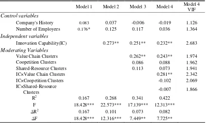
INNOVATION CAPABILITY AND PERFORMANCE IN TAIWANESE 80
SCIENCE PARKS: EXPLORING THE MODERATING EFFECTS OF INDUSTRIAL CLUSTERS FABRIC
Ming-Tien Tsai, Chung-Lin Tsai
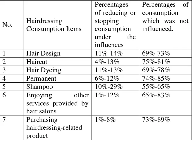
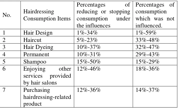
THE INFLUENCES OF THE FINANCIAL CRISIS ON THE 104 CONSUMPTION OF HAIRDRESSING IN TAIWAN
BOARD COMPOSITION AND CORPORATE VALUE IN TAIWAN 126 HIGH-TECHNOLOGY FIRMS
Derek TeShun Huang, Zhien Chia Liu
RESEARCH AND DEVELOPMENT ON THE APPLICATION OF TRIZ 139
INNOVATIVE PRINCIPLES TO BALANCED SAILBOAT PATENT Mean-Shen Liu, Sheu-Der Wu, Wen-Che Hong
A STUDY ON TAIWANESE ADULTS’COGNITION OF THE COLOR 160
COMBINATIONS OF HEALING TOYS An Sheng Lee, Jyun-Wei Wang
MODERATION OF GENDER ON THE RELATIONSHIP BETWEEN 195
TASK CHARACTERISTICS AND PERFORMANCE Setyabudi Indartono, Chun-Hsi Vivian Chen
AN EMPIRICAL STUDY ON THE IMPACT OF DIFFERENCES IN BED 223
AND BREAKFAST SERVICE QUALITY ATTRIBUTES ON CUSTOMERS’ REVISITING DESIRES
Wu-Chung Wu, Chih-Yun Yang
USING DATA MINING TO SOLVE FLOW SHOP 241
SCHEDULING PROBLEMS
Chinyao Low, Shiang-Huei Kung, Chikong Huang
---
The International Journal of Organizational Innovation (ISSN 1943-1813) is a blind peer- reviewed journal published online quarterly by The International Association of Organizational Innovation (IAOI). To Contact the Editor, email: drfdembowski@aol.com
For information regarding submissions to the journal, go to: http://ijoi.fp.expressacademic.org/ For more information on the Association, go to: http://www.iaoiusa.org
BOARD OF EDITORS 2010
! " # $ %
&
' # $ % ( %
& )! )!
* ! %
+ ! )!
, # $ %
- +& )!
' # $ %
) ! ) )!
, # $ % # "
! )!
* ! %
)
# $ % %
. /
# $ %
)! ! !
)! )! # $ %
! 0
1 !
, 2 * ! %
"
# ' 3
%
# $ % '
4
5 # $ %
6 % & !
# $ % %
! - &
! # $ %
, $
3 ! 1 !
# $ % ! )
*! " 1
Assistant Editors, Continued: ( # $ % ' ! 1 ! ! # $ % ( ! # $ %
7 + %
' 1 ! # $ %
"
6
) % # $ %
6 ! ( !
, # $ %
" ( 8
" 4 !
, !
( )
- # $ %
, ' %
9 # $ %
% ! ! # $ % ' ! # $ # ( % " % # $ % " , ) # $ % )!
! " # $ %
*
! " # $ %
! *
* 5 "2( # $ %
6 0 1 #
0 # $ % )! !
* 9 %
4 ) # $ %
-)! )! # $ %
.
! ) # $ %
! + 7 !
+ ! # $ %
' /" 7
# $ ( %
Government Administration Efficiency and Economic Efficiency
For 23 Districts in Taiwan
Yu-Chuan Chen, Department of Finance,
Chihlee Institute of Technology. Taiwan
ycchen@mail.chihlee.edu.tw.
Yung-Ho Chiu,
Business School, Soochow University. Taiwan
echiu@ scu.edu.tw.
Chin-Wei Huang, Soochow University, Taiwan
davy641126@yahoo.com.tw.
Abstract
In this study, the Seiford and Zhu (2002) undesirable modeling is used to measure the government and economic efficiencies of 23 counties or cities in Taiwan. We also carry on a correlation analysis upon the government and economic efficiencies. The data sources for this study consist of 23 counties or cities for the period from 2002 to 2005 as released by the Ministry of Economic Affairs of the R.O.C.
Our empirical results from the DEA (Data Envelopment Analysis)approach are
government efficiency, Taipei County, Taoyuan County, Hsinchu County, Changhua County, Nantou County, Yunlin County, Kaohsiung County, Pintung County, and Kaohsiung County rank at the worst level. (5) There is a positive relationship between economic efficiency and government efficiency. This result is consistent with Chen and Lee (2005).
Ke y Words: Data Envelopment Analysis, BCC, Undesirable Modeling, Government and Economic Efficienc y
Introduction
The market mechanism of pure capitalism can produce the most desired commodities
through the most efficient techniques. As a result, the capitalist system relies on the market
mechanism to allocate resources within economies. However, if the market mechanism fails to
allocate resources efficiently (called market failure), then the government must take part in the
economic system operation to adjust the market failure, by providing policy formulation and
guidance for the economic system’s development. In other words, the household (that buys the
commodities) and firm (that produces the commodities) sectors make up the economic activity
foundation for the most efficient allocation of resources. The government must also provide legal
and social frameworks and maintain competition and the reallocation of resources. Therefore,
households, businesses, and the government have mutual effects in the economic system.
department, the higher the efficiency is of an economic system that is created. With the
development of international and global financial markets, the current economic environment
faces severe challenges. A government plays a major role to influence its own economy’s
development under this environment. According to the 2007-2008 Global Competitiveness
Report, there are 12 pillars of competitiveness: Institutions, Macro-economy, Infrastructure,
Health and Primary Education, High Education and Training, Goods Market Efficiency, Labor
Market Efficiency, Financial Market Sophistication, Technological Readiness, Market Size,
Business Sophistication, and Innovation. In the first pillar, Institutions compose the framework
among households, firms, and governments that interact to create wealth in the economic system
and play an important role to achieve sustained economic growth and long-term prosperity. From
the annual Global Competitiveness Reports, except for Education, Financial market,
Technological, and Innovation, we know that economic efficiency and government efficiency
also are important ingredients in the Global Competitiveness index.
Taiwan’s 23 counties and cities in general currently have financial problems. In order to
solve these problems, the 23 counties and cities have adopted the enterprise managing concept to
promote government efficiency in order to improve their local business environment and
to promote local competition. Thus, the issues of government and economic efficiencies have
become more and more important.
The previous literature focuses mainly upon two major streams of research: (1) regional
economic efficiency and (2) government administration efficiency. Studies on regional economic
efficiency includes Charnes et al. (1989), Färe et al. (1994), Maudos et al.(2000), Martic and
Savic (2001), Afonso and Aubyn (2005), Timmer and Los (2005), Ma and Goo (2005), and
Mastromarco and Woitek (2006). Initially, the government is adopted as the input variable and
then is used to explain the efficiency scores. Instead of economic activity indicators, those who
take government expenditure as an input and infrastructure and the quality of life as outputs to
measure government administration efficiency are Hughes and Edwards (2000), Worthington
and Dollery (2002), Sun (2002), and Afonso and Fernandes (2006). From the above reviews we
see that most studies on government and economic efficiencies are discussed separately, but they
should be discussed together.
We also use the Seiford and Zhu (2002) DEA (Data Envelopment Analysis) undesirable
model to measure the government and economic efficiencies in order to improve performance.
Both desirable (good) and undesirable (bad) outputs and inputs may exist in a traditional DEA.
In the private sector, the production process may generate undesirable outputs like pollution or
undesirable outputs like crime for the estimation of government efficiency. If we do not consider
the undesirable (bad) outputs, then it does not reflect the true government and economic
efficiency
In this paper we first resort to the DEA model on discussing government and economic
efficiencies together for the 23 districts in Taiwan and carry on a correlation analysis between
the two efficiencies. Second, we use the Seiford and Zhu (2002) DEA undesirable model to
measure the government and economic efficiencies in order to avoid over-evaluation and
under-evaluation without consider the undesirable (bad) outputs. The structure of this paper is listed as
follows: Introduction, Literature Review, Methodology and Data Resources, Empirical Results
and Conclusion.
Literature Review
The efficiency performance of the economic unit is always paid attention to by economic
and management domain. Many scholars focus on the manufacturing sector and evaluate
efficiency with firm-level data. Two typical approaches are exploited. The first approach is using
a statistical method to estimate efficiency as developed by Battese and Coelli (1992; 1995). The
other approach is using the linear programming approach to measure a firm’s efficiency within
between regions or countries. They take regions or countries into the decision making units
(DMU) and measure their efficiency.
Charnes et al. (1989) used DEA to evaluate the economic efficiency of 28 cities in China in
1983-1984. The indictors of input are the number of employees, wage, and fixed asset
investment, and the indictors of output are the gross output value of industry, profit, tax, and
retail sales. The results show thatDEA could be used to identify technical inefficiencies and
related waste for each city’s economic activities in China.
Färe et al. (1994) took gross domestic product (GDP) as an output index, as well as capital
and employment as input indices, to analyze the efficiency of 17 countries in the OECD in
1978-1988. The results present that U.S. productivity growth is slightly higher than the average of 17
OECD countries, which is due to technical change. The highest productivity growth index is
Japan.
Maudos et al. (2000) measured the efficiency of 17 autonomous regions in Spain over 30
years. The indictors of input are labor and capital, and the indictor of output is gross value added.
The results show that the rich countries have experienced the greatest growth in TFP
(particularly through greater technical progress), and technical change has worked against labor
productivity convergence, since it has always been greater in countries with higher labor
Timmer and Los (2005) evaluated the economic efficiency of 40 countries around the
world. They took labor GDP production per unit as the input variable and labor capital per unit
as the output variable in 1975-1992. The results show that the change in the global production
frontier is localized at high levels of capital intensity and that the effect is stronger in agriculture
than in manufacturing.
Ma and Goo (2005) used capital and labor as input variables and revenue and profit as
output variables to assess the relative efficiency and total factor productivity (TFP) between the
53 High- and New-Technology Industry Development Zones (HNTIDZs) in China. The results
show that Xiamen, Chengdu, Huizhou, Wuxi, Shenzhen, Beijing, Shanghai, and Yangling
achieved technical efficiency. In comparison, the others were relatively inefficient and should
adjust according to input excesses and output deficits.
Under the category of macroeconomics, the government plays an important role in
economic growth and promotion of welfare. From the amount of regional economic efficiency
studies, how a government acts is also considered an important variable in efficiency
measurement.
Mastromarco and Woitek (2006) adopted the stochastic frontier approach (SFA) to estimate
the technical efficiency of 20 regions in Italia during 1970-1994. Except for labor and private
the percentage is of public capital stock divided by total capital stock, the more helpful it will be
to upgrade technical efficiency. Furthermore, some scholars take the quality indices of residents’
life and the scale of infrastructure instead of production and profit as the input variables when
they are estimating regional economic efficiency.
Martic and Savic (2001) estimated the efficiency of 30 regions in Serbia in 1979-1980 by
the CCR model. The four inputs include land, fixed assets, energy, and the quantity of
population, and the output takes up the quality indices of life, including the total number of
physicians, the total number of pupils in primary school, and the employed ratio.The results
show that 17 out of 30 regions are efficient, in which 5 regions are from Vojvodina and 12
regions are from central Serbia, while all regions from Kosovo and Metohia are inefficient.
Afonso and Aubyn (2005) compared the efficiency of education and medical treatment in
24 countries of the OECD by DEA application and free disposable hull (FDH) application. The
indicators of input are the numbers of teachers, doctors, nurses, and sickbeds. The indicators of
output are measured by the students’ performances of PISA, the average age, and the infant
survival rate. The results show that efficient outcomes across sectors and analytic methods seem
to cluster around a small number of core countries, (Japan, South Korea, and Sweden) even if for
input and infrastructure and the quality of life as outputs to measure government administration
efficiency in each locality.
Hughes and Edwards (2000) used the CCR and BCC models of DEA to evaluate the
efficiency of 73 Minnesota counties. The outputs are the total property value of the counties, and
the government expenditures of education, social services, transportation, public safety,
environmental protection, and administration. They considered the poverty rate, crime rate,
employment opportunities, water, and land area as input variables.The result indicates that the
dominant source of public sector inefficiency is an inappropriate scale of operations. It implies
that some counties’ jurisdictions are too large to serve the population efficiently, and that the size
and concentration of public power are also responsible in part for observed inefficiencies.
Worthington and Dollery (2002) employed the contextual and non-discretionary inputs
DEA to measure the relative efficiency of the 173 NEW local governments. The results show
that the number of councils assessed as perfectly efficiency.
Sun (2002) employed the output-oriented BCC model to measure the relative efficiency of
the 14 police administrators in Taipei city. The indicators of input include the expenditure of
police administrators, the numbers of police officers employed, the number of civilians
employed, and the equipment assets used by the police. The indicators of output include the
emergency. The results show that differences in operating environment, such as resident
population and location factors, do not have a significant influence upon the efficiency of police
precincts.
Afonso and Fernandes (2006) discussed local government efficiency from the view of
administration servers, education, social activity, and environment protection. They used the
DEA-BCC model to measure the expenditure efficiency of 51 local governments of Portugal in
2001. The input uses the total expenditures of the local governments. The indictors of output
include the number of residents and schools, social services for elders, the amount of clean water
supplied, the cleaning and carrying of litter, and the amount of recycling. The results show that
the 51 municipalities could have achieved, on average, roughly the same level of local output
with about 41% fewer resources - i.e. local performance could be improved without necessarily
increasing municipal spending.
Through a look at the previous studies, we know that the scope of research in efficiency
extends from the analysis between firms or enterprises to countries or areas. The categories of
efficiency are economic efficiency and government efficiency. However, the relationship
between economic efficiency and government efficiency is still seldom discussed in past years
and now we turn to focus on this point of view.
Methodology
Ever since Farrell (1957) proposed the concept of the frontier function to measure efficiency, many scholars have used linear programming or the frontier function method to estimate
efficiency and productivity. Charnes et al. (1978) extended Farrell’s model to multiple
inputs-outputs pattern and employed mathematical programming to develop an efficient frontier and to
estimate the efficiency score. This approach is named “Data Envelopment Analysis (DEA)”. The
Charnes, Cooper, and Rhodes (CCR) efficiency concept is subject to the strong hypothesis of
constant returns to scale. Banker, Charnes, and Cooper (BCC) proposed a variable returns to
scale model. The BCC model can determine the returns to scale for each DMU. The BCC models
can be formulated as:
n j z z y s y z x s x z t s j n j j n j j j n j j j , , 1 , 0 , 1 , . . : max 1 1 0 1 0 = ≥ = = − = + = = + = −
θ
θ
Here, θ is the score of the DMU, yjis the j-th output, xj is the j-th input, zj is the weight of the
In the methodology we know that the traditional DEA (CCR or BCC) model relies on the
assumption that inputs have to be minimized and outputs have to be maximized. However, many
production processes may produce undesirable outputs, such as the number of defective products, waste, and pollution. In other words, there exist desirable (ygj ) and undesirable (
b j y )
outputs. Obviously, desirable outputs should be increased and undesirable outputs should be
decreased in order to improve efficiency. However, the undesirable outputs should be increased
rather than decreased in the traditional DEA assumption, but they do not conform to the
isotonicity characteristic results in the inaccurate efficiency estimates. Charnes et al. (1985)
treated the undesirable outputs as inputs so that the bad outputs can be reduced. Seiford and Zhu
(2002) believed that treating the undesirable outputs as inputs does not reflect the true production
process. Hence, Seiford and Zhu (2002) proposed an approach to treat undesirable input/outputs
in the VRS envelopment. This approach follows the “classification invariance’ concept in Ali
and Seiford (1990) to deal with the problem of undesirable outputs. Following the Seiford and
Zhu (2002) undesirable model, the matrix can be presented as follows:
− = −
X Y Y X
Y b
g .
The terms g
Y and b
Y represent the corresponding desirable and undesirable outputs and X represents the input. It is clear that we desire to increase the desirable outputs ( g
decrease the undesirable outputs ( b
Y ) to improve efficiency. Thus, we multiply each undesirable output by (-1) and then find a proper value w to convert negative data to positive
(ybj =−ybj +w>0) data and maintain the invariant to the data. Employing the previous
notations, the model is:
n j z z x x z y y z y y z t s j n j j n j j j n j b b j j n j g g j j , , 1 , 0 1 . . : max 1 1 0 1 0 1 0 = ≥ = ≤ ≥ ≥ = = = =
θ
θ
θ
Here, θ is the score of the DMU, ygj and b j
y correspondingly represent the j-th desirable and undesirable outputs, xj is the j-th input, and zj is the weight of the j-th DMU.
Data Collection and the Chosen Outputs and Inputs
Data Collection
Taiwan is divided into 23 different districts and mainly into four regions named Northern,
Central, Southern, and Eastern. The Northern region has Taipei City, Keelung City, Hsinchu
City, Taipei County, Taoyuan County, Hsinchu County, and Ilan County, the Central region has
Yunlin County, the Southern region includes the 8 districts of Kaohsiung City, Tainan City,
Chiayi City, Chiayi County, Tainan County, Kaohsiung County, Pintung county, and Penghu
County, while the Eastern region includes the 2 counties of Hualien and Taitung. The data
sources for this study consist of 23 counties or cities for the period from 2002 to 2005 as released
by the Ministry of Economic Affairs of the R.O.C. The pertinent definitions of the variables, as
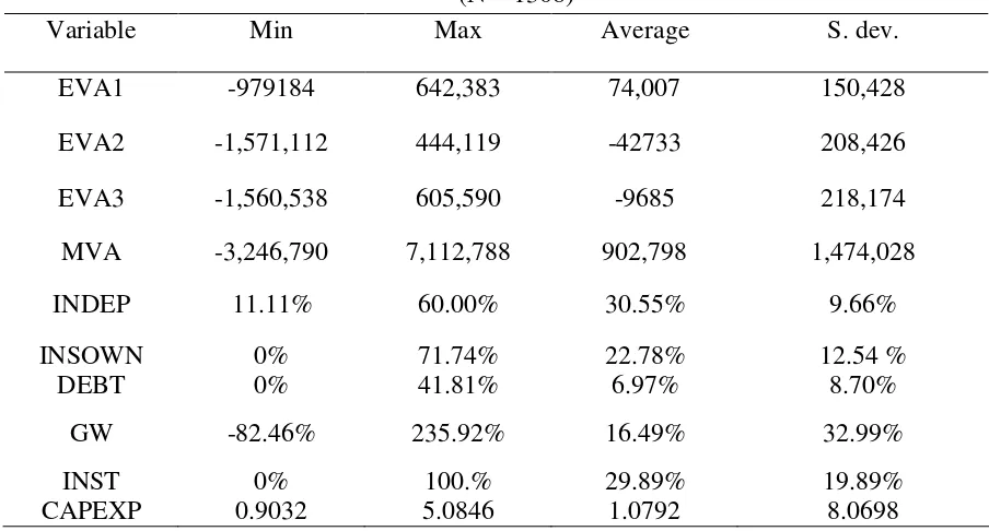
well as the original data and explanations of the data, are described in Table 1.
The Chosen Outputs and Inputs
A. Economic Efficiency
The major indicators used to measure Economic Efficiency include GDP (Fare et al 1995;
Martic and Savic, 2001; Timmer and Los, 2005), Industry output (Charnes et al, 1989), and its
side benefits (Maudos et al, 2000; Percoco, 2004). This research uses the sales income of each
registered company at the Ministry of Finance in each division as output variables (EY1). Due to
global warming and the rise of environmental protection, environmental pollution needs to be
considered when measuring the output of economic efficiency. Arcelus and Arocena (2005) used
the control of carbon dioxide amount as an output item, while Fare et al. (2004) took carbon
dioxide and three other green gases as undesirable output. The major indicators that Taiwan’s
region uses for air pollution include dust volume, sulfur dioxide, ozone, and thickness of RSP.
power products, factory pots, and flare gas for auto and motor transportation. The more
economic development grows, the higher the pollution increases. This research uses the
thickness of sulfur dioxide and ozone detected in districts by the Environmental Protection
Administration by as pollution output (EY2) index and takes it as the undesirable output in scale.
Among the inputs of economic efficiency, assets and labor are the main indicators of
economic activities (Maudos et al, 2000; Martic and Savic, 2001; Percoco, 2004). This research
will implement the assets of the companies registered at the Ministry of Economic Affairs as the
asset input (EXI), while the labor input (EX2) is made up of statistics on 15 years old and above
income labor and the number of people and non-income indoor labor who work 15 hours or more
in every district gathered by the Directorate-General of Budget, Accounting, Statistics, Executive
Yuan. In addition, the dimension of the land might affect the road scale, population density, and
number of buildings, and they are identified as input variables in most research studies (Hughes
and Edwards, 2000; Martic and Savic, 2001; Ma and Goo, 2005). According to the land
dimension announced by the Ministry of Administration, the land dimension has adopted the
Urban Development Plan Region as its main land input variables (EX3), by considering the
incapability of commercial activity in mountains, rivers, and valleys.
On the evaluation on government efficiency, the research of Sun (2002), Hughes and
Edwards (2002), and Afonso and Fernandes (2006) took government expenses as the
government efficiency input indicator. This article herein is based on annual income sources
(which include incoming financial sources, federal subsidy, and loans) that are announced by the
Ministry of Statistics as the Government Efficiency index (GX1).
Public construction (Percoco, 2004; Afonso and Fernsndes, 2006) and citizens’ living
environment are the main output performances for government. The criteria to evaluate living
environment quality includes security (Sun, 2002), education, medication (Afonso and Aubyn,
2005), social welfare (Afonso and Fernandes, 2006), and so on. Not only does this index indicate
the regional habitation living quality, it also reflects the quality of its commercial environment.
This research uses the percentage of social welfare staff among total population in each district
to observe the government’s performance in practicing social works among total population
(GY1), 15 years old and above who receive a higher education rate (GY2) as education
performance, and the population of medical practicing staff to evaluate the resources of medical
support index.
To increase the convenience of civil activities, the urban plan usually sets up space for
public commendation, which is divided and based upon population, use of land, traffic
using public commendation land dimension for over 10,000 people (GY4) shows the
government’s contribution in public commendation performance. The output index for public
security is evaluated by crimes committed, thefts, and violent crime detection rate (GY5), and
takes crime detection rate as the undesirable output.
Table 1. Variable Descriptions Variables Term Description
Asset EX1 Current Companies’ Registered Assets (NT$ million) Labor EX2 Working Population (Thousand)
Land EX3 Urban Plan Dimension
Economics
Output EY1 Sales Income (NT$ million)
Pollution EY2 Thickness of Sulfur Dioxide and Ozone (ppb) in Air Government
Output GX1 Annual Output (NT$ million)
Social Work GY1 Social Welfare Workers Among Total Population (%) Education GY2 Education Rate of 15 Year Olds & Above in Population
(%) Public
Commendation GY3
Land Dimension for Urban Plan on Public Space / 10,000 People (ha.)
Medical GY4 Population of Medical Staff Over All the Population (%) Public Security GY5 Crime, Theft, Violent-Crime Detection Rate (%)
Table 2 lists various indicators for statistical description. In Table 2, we naturally find
the most thriving economic activities are in Taipei City and Taipei County. Here, assets, working
population, and commercial sales income all reach a very high rate, but the two with their high
density of commercial activities sacrifice the living space of their citizens. The low economic
population, Chiayi County and Tainan County receive more social welfare or medical resources.
The less industrialized these areas are, the more the local government can promote tourism and
also create more recreational space for the local citizens.
Table 2. Descriptive Statistics of Variables in this Study (2002-2005)
EX1 EX2 EX3 EY1 EY2 GX1 GY1 GY2 GY3 GY4 GY5
2002 Mean 675,245 411 196 1,071,600 28 28,699 6 23 16 0.008 66
Std.Dev. 1,669,030 356 241 1,886,560 7 29,236 5 9 6 0.003 12
Max. 8,164,310 1,562 1,209 8,886,940 38 145,159 21 48 27 0.015 88
Min. 4,109 32 11 18,353 0 6,357 1 10 8 0.004 46
2003 Mean 702,040 416 196 1,188,800 29 32,008 7 25 16 0.008 68
Std.Dev. 1,731,190 360 241 2,123,020 7 31,966 5 9 6 0.003 11
Max. 8,454,980 1,578 1,209 10,015,800 39 149,100 19 48 27 0.015 85
Min. 4,127 33 10 17,956 0 6,898 1 11 8 0.004 50
2004 Mean 724,668 426 196 1,390,070 31 35,470 7 26 16 0.008 66
Std.Dev. 1,768,850 370 241 2,467,590 8 34,502 4 9 6 0.003 12
Max. 8,633,830 1,628 1,210 11,708,500 40 160,405 20 50 27 0.015 86
Min. 4,159 34 10 19,613 0 7,389 1 12 8 0.005 44
2005 Mean 753,297 432 196 1,491,190 30 35,858 7 27 16 0.009 66
Std.Dev. 1,827,660 377 241 2,747,980 7 34,873 4 9 6 0.003 13
Max. 8,921,530 1,664 1,210 13,126,300 38 158,151 16 52 27 0.016 87
Min. 4,010 34 10 21,784 0 6,841 1 13 8 0.005 48
Empirical Results
Efficiency Analysis
This research employs the computer program DEA Excel Solver to estimate Seiford and
From Table 3, in 2002 the average economic efficiency value is 0.913 and the average
government efficiency value is 0.901. In 2003 the average economic efficiency value is 0.910
and the average government efficiency value is 0.913. In 2004 the average economic efficiency
value is 0.908 and the average government efficiency value is 0.905. In 2005 the average
economic efficiency value is 0.859 and the average government efficiency value is 0.889. The
measurement results yielded by economic efficiency and government efficiency have no
apparent difference. Furthermore, economic and government efficiencies show that they
gradually decline annually.
For economic efficiency, Taipei City, Taichung City, Tainan City, Chiayi City, Taitung
County, Hualian County, and Penghu County are always on the frontier of DEA. Taichung
County, Tainan County, Chiayi County, Yilan County, and Hsinchu City take second place.
Nantou County, Miaoli County, Kaohsiung City, Taipei County, and Taoyuan County rank the
worst level.
In government efficiency, the efficiency scores of Taipei City, Taichung City, Tainan City,
Chiayi City, Taitung County, Hualian County, and Penghu County are all 1 in the DEA
estimation, thus ranked #1. Keelung City places 11th in 2002 and 2003, but progresses the best in
government efficiency among all areas after 2004. Pintung County, Yunlin County, Kaohuiung
Economic Efficiency and Government Efficiency Analysis
The Quadrant
In order to have a better understanding of the relationship between economic efficiency and
government efficiency for each county or city, we use the quadrant to graphically show the
position of each county or city.
We divide the quadrant with government efficiency as the vertical axis and economic
efficiency scores as the horizontal axis. In this research we plot the quadrant according to the
efficiency scores under Seiford and Zhu’s (2002)undesirable models. Thus, the vertical axis
offers the average government efficiency scores, which means the county or city located to the
right side of the vertical axis possesses a higher government efficiency on average in the county
or city. The horizontal axis presents the average economic efficiency scores, which means the
county or city located above the horizontal axis possesses a higher economic efficiency on
average in the county or city. Quadrant I represents higher economic efficiency and higher
government efficiency. Quadrant II represents higher economic efficiency and lower government
efficiency. Quadrant III represents lower economic efficiency and lower government efficiency.
Quadrant IV represents lower economic efficiency and higher government efficiency (see Figure
Table 3. Economic Efficiency and Government Efficiency
2002 2003 2004 2005 Average
Econ. Eff. Gov. Eff. Econ. Eff. Gov. Eff. Econ. Eff. Gov. Eff. Econ. Eff. Gov. Eff. Econ. Eff. Gov. Eff. Score R Score R Score R Score R Score R Score R Score R Score R Score R Score R
Taipei County 0.809 22 0.701 23 0.761 23 0.698 23 0.745 23 0.676 23 0.715 22 0.703 22 0.758 23 0.695 23
Yilan County 0.912 11 0.888 12 0.900 13 0.929 12 0.931 10 0.920 12 0.911 11 0.911 11 0.914 11 0.912 12
Taoyuan County 0.787 23 0.824 19 0.785 22 0.834 19 0.774 22 0.812 19 0.695 23 0.743 21 0.761 22 0.803 19
Hsinchu County 0.910 12 0.923 10 0.995 9 1.000 1 0.861 14 0.860 17 0.816 18 0.787 19 0.895 13 0.892 14
Miaoli County 0.822 20 0.875 15 0.805 21 0.922 14 0.838 20 1.000 1 0.838 16 0.955 10 0.826 21 0.938 10
Taichung County 0.943 10 0.975 9 0.935 11 0.975 9 0.896 12 0.859 18 0.848 15 0.846 16 0.906 12 0.914 11
Changhua County 0.867 14 0.853 16 0.854 16 0.884 16 0.842 18 0.871 15 0.849 14 0.878 12 0.853 16 0.871 16
Nantou County 0.835 19 0.836 17 0.830 19 0.913 15 0.837 21 0.893 13 0.814 20 0.827 17 0.829 20 0.867 17
Yunlin County 0.855 18 0.763 21 0.808 20 0.732 22 0.841 19 0.791 21 0.834 17 0.796 18 0.835 19 0.770 21
Chiayi County 0.960 9 0.884 13 0.946 10 0.924 13 0.964 9 0.938 11 0.966 9 0.857 14 0.959 9 0.901 13
Tainan County 1.000 1 0.881 14 1.000 1 0.871 17 0.999 8 0.876 14 0.972 8 0.870 13 0.993 8 0.875 15
Kaohsiung County 0.860 16 0.810 20 0.860 15 0.803 20 0.859 15 0.806 20 0.815 19 0.777 20 0.849 17 0.799 20
Pintung County 0.861 15 0.747 22 0.839 17 0.751 21 0.844 17 0.710 22 0.890 12 0.671 23 0.859 15 0.720 22
Taitung County 1.000 1 1.000 1 1.000 1 1.000 1 1.000 1 1.000 1 1.000 1 1.000 1 1.000 1 1.000 1
Hualien County 1.000 1 1.000 1 1.000 1 1.000 1 1.000 1 1.000 1 1.000 1 1.000 1 1.000 1 1.000 1
Penghu County 1.000 1 1.000 1 1.000 1 1.000 1 1.000 1 1.000 1 1.000 1 1.000 1 1.000 1 1.000 1
Keelung City 0.859 17 0.922 11 0.864 14 0.953 11 0.859 16 1.000 1 0.862 13 1.000 1 0.861 14 0.969 9
Hsinchu City 0.893 13 1.000 1 0.917 12 0.956 10 0.913 11 0.943 10 0.955 10 0.985 9 0.920 10 0.971 8
Taichung City 1.000 1 1.000 1 1.000 1 1.000 1 1.000 1 1.000 1 1.000 1 1.000 1 1.000 1 1.000 1
Chiayi City 1.000 1 1.000 1 1.000 1 1.000 1 1.000 1 1.000 1 1.000 1 1.000 1 1.000 1 1.000 1
Tainan City 1.000 1 1.000 1 1.000 1 1.000 1 1.000 1 1.000 1 1.000 1 1.000 1 1.000 1 1.000 1
Taipei City 1.000 1 1.000 1 1.000 1 1.000 1 1.000 1 1.000 1 1.000 1 1.000 1 1.000 1 1.000 1
Kaohsiung City 0.821 21 0.831 18 0.839 18 0.847 18 0.869 13 0.868 16 0.814 21 0.849 15 0.836 18 0.849 18
Mean 0.913 0.901 0.910 0.913 0.908 0.905 0.895 0.889 0.907 0.902
Std.Dev. 0.076 0.094 0.085 0.095 0.082 0.098 0.096 0.108 0.082 0.095
Maximum 1.000 1.000 1.000 1.000 1.000 1.000 1.000 1.000 1.000 1.000
From Figure 2, we find that there are 8 counties or cities, 11 counties or cities, 10
counties or cities, and 9 counties or cities in Quadrant I in 2002, 2003, 2004, and 2005,
respectively. There are 2 counties or cities, 1 county or city, 1county or city, and 2 counties or
cities in Quadrant II in 2002, 2003, 2004, and 2005, respectively. There are 10 counties or cities,
7 counties or cities, 10 counties or cities, and 10 counties or cities in Quadrant III in 2002, 2003,
2004, and 2005, respectively. There are 1 county or city, 4 counties or cities, 2 counties or cities,
and 3 counties or cities in Quadrant III in 2002, 2003, 2004, and 2005, respectively.
The Distribution of 23 Counties or Cities
We choose those counties or cities which remained in the same quadrant for four years as
the representatives of Quadrants I, II, III, and IV (see Table 4).
Ⅰ Ⅰ Ⅰ Ⅰ
Economic Efficiency Government
Efficiency
Ⅲ Ⅲ Ⅲ
Ⅲ ⅣⅣⅣⅣ
Figure 1. The quadrant
Figure 2 Economic Efficiency and Government Efficiency Distribution Map (2002-2005)
1. Quadrant I: These counties or cities are operating efficiently and have high economic
efficiency and high government efficiency compared to others. We see that most of the counties
or cities in this area are those with a mature commercial development or well-known as leaders
in the tourism industry. The representative counties or cities include Taipei City, Hsinchu City,
Taitung City, Chiayi City, Tainan City, Yilan County, Taitung County, Hualian County, and
Penghu County. 0.500
0.600 0.700 0.800 0.900 1.000
0.750 0.800 0.850 0.900 0.950 1.000
0.500 0.600 0.700 0.800 0.900 1.000
0.750 0.800 0.850 0.900 0.950 1.000
0.500 0.600 0.700 0.800 0.900 1.000
0.750 0.800 0.850 0.900 0.950 1.000
0.500 0.600 0.700 0.800 0.900 1.000
0.750 0.800 0.850 0.900 0.950 1.000
2003 2005
government efficiency. If they properly adjust government performance, then they may also
upgrade to compete with those counties or cities in Quadrant I. The representatives of Quadrant
II are Chiayi County and Tainan County.
3. Quadrant III: These counties or cities are operating inefficiently and have lower
economic efficiency and lower government efficiency. The representative counties or cities are
Taipei County, Taoyuan County, Hsinchu County, Changhua County, Nantou County, Yunlin
County, Kaohsiung County, Pintung County, and Kaohsiung city. These counties or cities should
adjust government management and change their operations to improve their performance.
4. Quadrant IV:These counties or cities have lower economic efficiency and higher
government efficiency. The representatives of Quadrant IV are Keelung City, Miaoli County, and
Taichung County.
From all of the above, we conclude that the counties or cities in Quadrant I perform the best
in each year while counties or cities in Quadrant III perform the poorest. The counties or cities in
Quadrants II and IVshow not many differences between them in some years.
Correlation Between Economic Efficiency and Government Efficiency
It is crucial to test if there is a high correlation between economic efficiency and
government efficiency. Here, we adopt the Pearson Correlation Coefficients Test, and the results
Table 4. The Distribution of Economic Efficiency and Government Efficiency in Quadrants
Higher Economic Efficiency Lower Economic Efficiency Taipei City Hsinchu City Keelung City
Taitung City Chiayi City Miaoli County
Taichung County Higher
Government Efficiency
Chiayi County Taipei County Yunlin County Tainan County Taoyuan County Kaohsiung County
Hsinchu County Pintung County
Changhua County Kaohsiung City Lower
Government Efficiency
Nantou County
efficiency are highly correlated with each other. In 2002 the economic and government efficiency
correlation coefficients are 0.789. In 2003 the two efficiency correlation coefficients are 0.800. In
2004 the two efficiency correlation coefficients are 0.742. In 2005 the two efficiency correlation
coefficients are 0.763.Thus, there exists a significantly positive correlation between economic
efficiency and government efficiency. This result is consistent with the result in Chen and Lee
(2005).
Table 5. Pearson Correlation Coefficients Econ. Eff.
2002 2003 2004 2005 Average
Gov. Eff. 2002 0.789 **
2003 0.800 **
2004 0.742 **
2005 0.763 **
Average 0.785 **
From the above analyses, we know that higher economic efficiency will be able to bring
about higher economical development, which simultaneously will be able to bring more sources
of wealth to the government and result in higher government efficiency. In other words,
government efficiency and economic efficiency complement one another and are able to create
areas that can be more prosperous.
Conclusion
Most studies in the existing literature have discussed government and economic
efficiencies separately, but they do not take them into account together. In this study we adopt
the Seiford and Zhu (2002) undesirable modeling to discuss government and economic
efficiencies together for 23 different districts in Taiwan and carry on the correlation analysis to
government and economic efficiencies. The conclusions of this paper are as follows.
1. The regions with the most thriving economic activities are Taipei City and Taipei County,
while low economic activity areas include Penghu County, Taitung County, Chiayi County, and
Tainan County.
2. Economic efficiency and government efficiency have no apparent difference. They also
show that economic and government efficiencies gradually decline annually
3. Taipei City, Hsinchu City, Taitung City, Chiayi City, Tainan City, Yilan County, Taitung
government efficiency compared to others. Most of the counties or cities are those with mature
commercial development or well-known as leaders in tourism.
4. Taipei County, Taoyuan County, Hsinchu County, Changhua County, Nantou County, Yunlin
County, Kaohsiung County, Pintung County, and Kaohsiung city have lower economic efficiency
and lower government efficiency.
5. Chiayi County and Tainan County have higher economic efficiency and lower government
efficiency. Keelung City, Miaoli County, and Taichung County have lower economic efficiency
and higher government efficiency
6. There is a positive relationship between economic efficiency and government efficiency. Thus,
higher economic efficiency is able to bring higher economical development, resulting in higher
government efficiency. This result is consistent with Chen and Lee (2005).
References
Afonso, A. and M. S. Aubyn, (2005), “Non-Parament Approaches to Education and Health Efficiency in OECD Countries,” Journal of Applied Economics, 8, 2, 227-246.
Afonso, A. and S. Fernandes, (2006), “Measuring Local Government Spending Efficiency: Evidence for the Lisbon Region,” Regional Studies, 40, 1, 39-53.
Arcelus, F. J. and P. Arocena, (2005), “Productivity Differences across OECD Countries in the Presence of Environmental Constraints,” Journal of the Operational Research Society, 56, 1352-1362.
Banker, R. D., A. C. Charnes, and W. W. Cooper, (1984), “Some Models for Estimating
Technical and Scale Inefficiencies in Data Envelopment Analysis,” Management Science, 30, 1078-1092.
Battese, G. E., and T. J. Coelli, (1992), “Frontier Production Functions, Technical Efficiency and Panel Data: With Application to Paddy Farmers in India,” Journal of Productivity
Analysis, 3, 153-169.
Battese, G. E., and T. J. Coelli, (1995), “A Model for Technical Inefficiency Effects in a
Stochastic Frontier Production Function for Panel Data,” Empirical Economics, 20, 325-32.
Charnes, A. C., W. W. Cooper, and E. L. Rhodes, (1978), “Measuring the Efficiency of Decision Making Units,” European Journal of Operational Research, 2, 429-444.
Charnes, A. C., W. W. Cooper, and S. Li, (1989), “Using Data Envelopment Analysis to Evaluate Efficiency in the Economic Performance of Chinese Cities,” Socio-Economic Planning Sciences, 6, 325-344.
Chen, S. T. and C. C. Lee, (2005), “Government Size and Economic Growth in Taiwan: A Threshold Regression Approach,” Journal of Policy Modeling, 27, 1051-1066. Färe, R., S. Grosskopf, C. A. Lovell, and C. Pasurka, (1989), “Multilateral Productivity
Comparisons when Some Outputs are Undesirable: A Nonparametric Approach,” The Review of Economics and Statistics, 71, 90-98.
Färe, R., S. Grosskopf, and M. Norris, (1994), “Productivity Growth, Technical Progress, and Efficiency Change in Industrialized Countries,” The American Economic Review, 84, 1, 66-83.
Farrell, M. J., “The Measurement of Productive Efficiency,” Journal of the Royal Statistical Society, 120, 3, 253-290.
Golany, B. and Y. Roll, (1989), “An Application Procedure for DEA,” OMEGA, 17, 237-250.
Hailu, A. and T. S. Veeman, (2001), “Non-Parametric Productivity Analysis Undesirable
Outputs: An Application to the Canadian Pulp and Paper Industry,” American Journal of Agricultural Economics, 83, 3, 605-616.
Hughes, P. A. and M. E. Edwards, (2000), “Leviathan vs. Lilliputian: A Data Envelopment Analysis of Government Efficiency,” Journal of Regional Science, 40, 2, 649-669
Li, Y., (2005), “DEA Efficiency Measurement with Undesirable Outputs: An Application to Taiwan’s Commercial Banks,” International Journal of Services Technology and Management, 6, 6, 544-555.
Ma, Y. F. and Y. J. Goo, (2005), “Technical Efficiency and Productivity Change in China’s High- and New-Technology Industry Development Zones,” Asian Business & Management, 4, 331-355.
Martic, M. and G. Savic, (2001), “An Application of DEA for Comparative Analysis and
Ranking of Regions with Regards to Social-Economic Development,” European Journal of Operational Research, 132, 343-356.
Mastromarco, C. and U. Woitek, (2006), “Public Infrastructure Investment and Efficiency in Italian Regions,” Journal of Productivity Analysis, 25, 1, 57-65.
Maudos, J., J. M. Pastor, and L. Serrano, (2000), “Efficiency and Productive Specialization: An Application to the Spanish Regions,” Regional Studies, 34, 9, 829-842.
Percoco, M., (2004), “Infrastructure and Economic Efficiency in Italian Regions,” Networks and Economics, 4, 361-378.
Sun, S., (2002), “Measuring the Relative Efficiency of Police Precincts Using Data Envelopment Analysis,” Socio-Economic Planning Sciences, 36, 51-71.
Timmer M. P. and B. Los, (2005), “Localized Innovation and Productivity Growth in Asia: An Intertemporal DEA Approach,” Journal of Productivity Analysis, 23, 47-64.
Worthington, Andrew c. and Brian E. Dollery (2002), “Incorporating Contextual Information in Public Sector Efficiency Analysis: a Comparative Study of NSW Local Government,” Applied Economics, Vol 34, 453-464.
THE APPLICATION OF FUZZY LINGUISTIC SCALE ON INTERNET
QUESTIONNAIRE SURVEY
Kuo-Ming Chu
Cheng Shiu University, Taiwan
Chu@csu.edu.tw
Abstract
The growing number of respondents with access to the internet introduces a new data collection alternative that is likely to become increasingly important in the future. The purpose of this paper is to develop the process of a fuzzy linguistic scale to solve the linguistic scale transformation problems generated by the traditional quantitative methods based on the Likert scale and semantic scale, and to reduce the difficulties of answering the fuzzy questionnaire. Therefore, the problem of dilution of measuring results due to the traditional linguistic value in which every scale interval is equal can be solved by using the fuzzy linguistic scale.
Introduction
measuring scale, often is ignored intentionally or unintentionally.
However, the studies conducted by Bradley, Katti, & Coons (1962) and Bradley (2006) suggest that the distance within the measuring scale usually is not set equally. Studies conducted by scholars domestically and internationally also show that an equal-distance scale unavoidably produces an incorrect estimate of factors. The use of fuzzy set theory, proposed and developed by Zadeh (1993), has given very good results modeling the qualitative aspects in linguistic terms.
Literature
Fuzzy Questionnaire Styles
In many social science studies, the purpose usually is to analyze concepts or attitudes of human beings. In this type of study, answers provided are not strictly “true” or “false,” due to some uncertainties of human behavior. Boolean Logic (Fuzzy Logic), on the contrary, takes into account the complexity of human thinking and uncertainties of human behavior.
used fuzzy theory to analyze service quality assessment. Lien & Chen (2005) applied fuzzy linguistic scale approach and discrete choice theory for building the housing consumption choice behavior model in a household. However, for the general public, it’s hard to draw lines to express attitudes and opinions. As Zadeh (1993) said using values to accurately decide relating and influential disciplines is not an easy task in many situations. A practical way is to establish a reference system. For instance, traditional questionnaires request test takers to write down “levels of attitude” on the scale to enable researchers to establish membership functions. This way, however, will increase the level of complexity of data collecting and calculations. It is not the most practical method in this aspect.
Fuzzy Linguistic Scale
To ask questionnaire takers to express their attitudes verbally is the easiest and the most direct method. But, researchers must be able to transform verbal expressions into values to expedite statistical analysis. In fuzzy theory studies, researchers often use fuzzy values to measure linguistic terms. Chen and Hwang (1992) offer a method of applying fuzzy theory to convert fuzzy numbers into crisp numbers.
will occur when the method is applied directly without considering the difference. Based on the above reasons, we provide a both practical and realistic fuzzy linguistic scale to construct processes to eliminate the problems embedded in Chen and Hwang’s method.
The Process
In our research, we build a process of fuzzy linguistic scale according to unequal scale intervals, different individuals, and disregard the inflated.
Step 1: Design a fuzzy linguistic scale questionnaire
Step 1.1 Decide the number of terms used
The verbal terms used in our scales are in the universe X={x1, x2, …,xm}; m is the number of
terms used.
Step 1.2 Decide the styles of linguistic combination
According to linguistic terms, there will be
(
)
2
1 m
m− ×
types of combination.
Step 2: Convey the scale questionnaire
Step 2.1 Analyzing the types of the questionnaire takers’ answers
After the answers of the key questionnaires are obtained, analyze the types of the scales
used by questionnaire takers according to overall scales shown. Design and distribute linguistic
questionnaires after the types of scales that contain minimum linguistic terms are obtained.
Step 2.2 Establish membership function belonged to individual test-taker
Define the linguistic terms variables (k) in questionnaires according to each individual’s (i) answers. Also, in an interval scale (0-1), subjectively determine the scope of linguistic terms by
( )
− − ≤ ≤ ≤ ≤ ≤ ≤ − − = o , 0 , , , 。 thers d x b d b d x w b x a w a x c c a c x wx ik ik ik ik ki
ki ik ki ik ik ik ik
Aik
µ (1)
Since,
Step 3: Integrate various types of linguistic scales
Integrating various types of linguistic variables should be done after the questionnaire
taker’s linguistic terms variable k is transformed into
A
ik , for different questionnaire takers ihave different recognition and experience. Kacprzyk et al. (1992), Ishikawa et al. (1993) and Hsu
& Chen (1996) proposed the formula of Fuzzy Delphi method to aggregate group opinions. But
this paper considers the participants to be many, and moreover the linguistic cognition is
different, it therefore uses the mean value to carry on the opinion integration, avoiding various
linguistic cognition scopes as too dispersing. Suppose the membership function of A is
A
k=(ck,ak, bk, dk)LR (4)
ck = 1 ,
n c
n
i ik
= (5)
n a a n i ik k =
= 1 (6)
n b b n i ik k =
= 1 (7)
n d d n i ik k =
= 1 . (8)
ki ik
ik ik
ik a c c x a
c x w x
L( ) = − − , ≤ ≤
ik ik
ik ik
ik b d b x d
d x w x
R( ) = − − , ≤ ≤
(2)
Step 4: Converting Fuzzy Number to Crisp Score
In the past, many scholars proposed the methods of defuzziness (Chen & Hwang, 1992;
Chen & Hsieh, 1998). At this stage, we adopted Chen & Hsieh’s (1998) method of defuzziness.
They proposed graded mean integration representation for a generalized fuzzy number. Now we
describe graded mean integration representation as follows:
Suppose L-1 and R-1 are inverse functions of functions L and R, respectively, and the
graded mean h level value of generalized fuzzy number A=(c, a, b, d; w)LR is h[L-1(h) +
R-1(h)]/2 as Figure 1. Then the graded mean integration representation of A is
( )= w − ( )+ − ( ) w
hdh h R h L h A P 0 0 1 1
2 (9)
Therefore, the formula (2) and (3) is modified as below:
Thus,
By formula (9), the graded mean integration representation of A is (Suppose A is a
trapezoidal fuzzy number). Since,
( )
( )
( )
6 2 2 2 0 0 1 1 d b a c hdh h R h L h AP w w
+ + + = + = − − (13)
A generalized triangular fuzzy number is a special case of generalized trapezoidal fuzzy
number when b=a. Then, replacing b by a in formula (13), the graded mean integration representation of A becomes
( ) ( ) ( ) 6 4 2 0 0 1 1 d a c hdh h R h L h A
P w w
+ + = + = − − (14)
According to this method, convert fuzzy numbers of linguistic terms to crisp scores. Then,
( )
( )
(
)
2 / 2 1 1 w h b d c a d c h R hL + + − − +
=
+ −
−
(12)
(
a
c
)
h
w
h
w
c
x
L
−1(
)
=
+
−
/
,
0
≤
≤
(
d
b
)
h
w
h
w
d
x
R
−=
−
−
≤
≤
after process reorganization, you can obtain the various types of linguistic terms’ translate table.
Case Study
Sampling Method and Sample Structure
The sample is including nine online communities in Taiwan, including Kimo, CPB, Sony
music etc. who were contacted and asked to participate in the study. Data were collected between
October and December 2008 via the web for Internet users using a standardized questionnaire.
First, a questionnaire of online helping behavior is handed to a online communities’ users.
Second, after the first questionnaire is completed, a second questionnaire containing linguistic
scale is handed to the online communities’ users.
Usually, answering a fuzzy linguistic questionnaire is not complicated. For this reason
and because not many samples will be needed, we design questionnaires for this study based on
representative samples. The method is that some random samples belonging to eight different
linguistic scale combinations are collected and investigated to derive at least 15 effective
samples for each linguistic scale.
Constructing Fuzzy Linguistic Scale
Based on consumer profit-segmentation variables, we first decide linguistic terms and
( ) 1( )/2
1 h R h
L− + − bR −1( )h
( )h cL−1
x d
a h
A
R(x)
expressed as X = (strongly agree, agree, normal, disagree, strongly disagree) five linguistic terms.
Next, forsake single linguistic scale and design ten combinations of linguistic scales, shown as
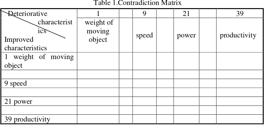
Table 1.
Table 1 The combinations of fuzzy linguistic scale
Types I II III IV V VI VII VIII IX X
Strongly Agree Yes Yes Yes Yes
Agree Yes Yes Yes Yes Yes Yes Yes
Normal Yes Yes Yes Yes Yes Yes Yes Yes
Disagree Yes Yes Yes Yes Yes Yes Yes
Strongly Disagree Yes Yes Yes Yes
Eliminate five questionnaires considered invalid out of the 130 questionnaires collected.
Sort remaining 125 questionnaires into different types. Based on the combinations of fuzzy
Integrating Various Types of Linguistic Scales.
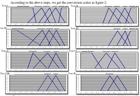
According to the above steps, we get the conversion scales as figure 2.
agree normal disagree
Type V
0 0 . 1 0 . 2 0 . 3 0 . 4 0 . 5 0 . 6 0 . 7 0 . 8 0 . 9 1
0 0 . 1 0 . 2 0 . 3 0 . 4 0 . 5 0 . 6 0 . 7 0 . 8 0 . 9 1
0 0 . 1 0 . 2 0 . 3 0 . 4 0 . 5 0 . 6 0 . 7 0 . 8 0 . 9 1
0 0 . 1 0 . 2 0 . 3 0 . 4 0 . 5 0 . 6 0 . 7 0 . 8 0 . 9 1
normal
strongly disagree disagree
Type VI
0 0 . 1 0 . 2 0 . 3 0 . 4 0 . 5 0 . 6 0 . 7 0 . 8 0 . 9 1
0 0 . 1 0 . 2 0 . 3 0 . 4 0 . 5 0 . 6 0 . 7 0 . 8 0 . 9 1
0 0 . 1 0 . 2 0 . 3 0 . 4 0 . 5 0 . 6 0 . 7 0 . 8 0 . 9 1
0 0 . 1 0 . 2 0 . 3 0 . 4 0 . 5 0 . 6 0 . 7 0 . 8 0 . 9 1
normal agree
0 . 5 0 . 6 0 . 7 0 . 8 0 . 9 1
0 . 5 0 . 6 0 . 7 0 . 8 0 . 9 1
Type VIII Type IX disagree
0 . 5 0 . 6 0 . 7 0 . 8 0 . 9 1
0 . 5 0 . 6 0 . 7 0 . 8 0 . 9 1
normal
Type I strongly disagree disagree agree strongly agree
0 0 . 1 0 . 2 0 . 3 0 . 4 0 . 5 0 . 6 0 . 7 0 . 8 0 . 9 1
0 0 . 1 0 . 2 0 . 3 0 . 4 0 . 5 0 . 6 0 . 7 0 . 8 0 . 9 1
0 0 . 1 0 . 2 0 . 3 0 . 4 0 . 5 0 . 6 0 . 7 0 . 8 0 . 9 1
0 0 . 1 0 . 2 0 . 3 0 . 4 0 . 5 0 . 6 0 . 7 0 . 8 0 . 9 1
agree normal disagree strongly disagree Type III 0 0 . 1 0 . 2 0 . 3 0 . 4 0 . 5 0 . 6 0 . 7 0 . 8 0 . 9 1
0 0 . 1 0 . 2 0 . 3 0 . 4 0 . 5 0 . 6 0 . 7 0 . 8 0 . 9 1
0 0 . 1 0 . 2 0 . 3 0 . 4 0 . 5 0 . 6 0 . 7 0 . 8 0 . 9 1
0 0 . 1 0 . 2 0 . 3 0 . 4 0 . 5 0 . 6 0 . 7 0 . 8 0 . 9 1
normal agree strongly agree
Type IV
0 0 . 1 0 . 2 0 . 3 0 . 4 0 . 5 0 . 6 0 . 7 0 . 8 0 . 9 1
0 0 . 1 0 . 2 0 . 3 0 . 4 0 . 5 0 . 6 0 . 7 0 . 8 0 . 9 1
0 0 . 1 0 . 2 0 . 3 0 . 4 0 . 5 0 . 6 0 . 7 0 . 8 0 . 9 1
0 0 . 1 0 . 2 0 . 3 0 . 4 0 . 5 0 . 6 0 . 7 0 . 8 0 . 9 1
normal
disagree agree strongly agree
Type II
0 0 . 1 0 . 2 0 . 3 0 . 4 0 . 5 0 . 6 0 . 7 0 . 8 0 . 9 1
0 0 . 1 0 . 2 0 . 3 0 . 4 0 . 5 0 . 6 0 . 7 0 . 8 0 . 9 1
0 0 . 1 0 . 2 0 . 3 0 . 4 0 . 5 0 . 6 0 . 7 0 . 8 0 . 9 1
individual logical thinking, effectively eliminating errors generated by a single conversion set.
linguistic scales, eliminate two types (VII and X) that no one used in our study. Design eight
different types of linguistic scale combinations. This method considers the difference in
Though there are only 12 and 13 questionnaires categorized into type V and IX, it is sufficient to
do linguistic scale analysis.
From Figure 2, the results are described as follows: First, thorough empirical
investigation obtained linguistic variables, various types of linguistic fuzzy numbers scale are
completely different, and presented the asymmetry. Namely, different linguistic types that the
fuzzy numbers present different values for the same linguistic terms. Second, from types 1 to 5,
we find that the general public tends to have consistent opinions regarding a linguistic term’s
more positive expression, namely, in “agree” and “very agree” on, participant's fuzzy number
chart width is narrow; namely, no matter whether the statement is the same, all had a close fuzzy
number graph. Finally, the fuzzy cognition of linguistic terms possesses “on the Double-sided
Property”. Namely, the fuzzy numbers of linguistic terms have an overlap phenomenon; for
example, the fuzzy numbers of “normal”, “agree,” and “strongly agree” possess the same
converting crisp scores under
α
-cuts=0.1
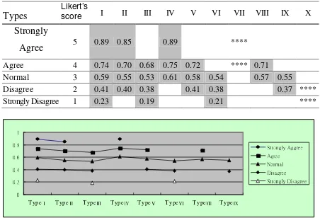
in type Converting Fuzzy Numbers to Crisp ScoresThen, according to the formula (13) and (14), convert each fuzzy number of Figure 1 to
crisp scores. From Table 2 and Figure 3, we quickly can obtain various type of linguistic terms’
crisp scores.
The question of equal distance of scales
From comparison in Table 2, it’s obvious that traditional questionnaires presuming equal
distance between scales assume everyone has same recognition levels when these levels are
has the same recognition levels. For instance, in type I, the transformed numbers are 0.89, 0.74,
0.59, 0.41, and 0.23, respectively.
Table 2 The various types of linguistic terms’ crisp scores and Likert’s score
Types
Likert’s
score I II III IV V VI VII VIII IX X
Strongly
Agree
5 0.89 0.85 0.89 ****Agree 4 0.74 0.70 0.68 0.75 0.72 **** 0.71
Normal 3 0.59 0.55 0.53 0.61 0.58 0.54 0.57 0.55
Disagree 2 0.41 0.40 0.38 0.41 0.38 0.37 ****
Strongly Disagree 1 0.23 0.19 0.21 ****
Figure 3 The types of linguistic terms’ crisp scores and Likert’s score
Comparison and Analysis
The questionnaire of single transformed value
When taking into account individuals’ different logical thinking, recognition levels will be
different as to a single linguistic term. Take “Agree” for example: traditional questionnaire is on
scale 4; on the other hand, the transformed values under Fuzzy Linguistic Scale are 0.74, 0.70,
0.68, 0.75, 0.72, and 0.71.
0 0.2 0.4 0.6 0.8 1
T ypeⅠ T ypeⅡ T ypeⅢ T ypeⅣ T ypeⅤ T ypeⅥ T ypeⅧ T ypeⅨ
Linguistic devaluation and inflation
Table 2 and Figure 3 show that we also have considered the phenomenon of linguistic
devaluation and inflation in human logical thinking. When using measurements containing lesser
scales, questionnaire takers tend to choose the “middle scale” and they would consider the width
of the scale when answering questionnaires. The phenomenon of linguistic devaluation and
inflation occurs frequently in the largest scale and the smallest scale sequentially.
The problem of dilution of measuring results
From Figure 3, the curve constituted by “average scale” values fluctuates most dynamically.
In traditional scales, assuming equal distance between scales, test takers tend to choose scales
closer to the middle one. Dilution of measuring results usually occurs. On the contrary, Fuzzy
Linguistic Scale is not equally distanced. It eliminates the problem presented by traditional
questionnaires by giving different linguistic terms and fuzzy values.
Conclusions
The Internet questionnaire method will become one of the major data collection methods in
the future research. According to this study, linguistic bias exists between the internet
questionnaire method and traditional method. We have the following conclusions for reference:
First, through a questionnaire, questionnaire takers are able to recognize the scope of linguistic
variables. The designed fuzzy linguistic conversion scale is able to solve the problem of
subjectively set membership function. The traditional type of questionnaire assumes distances
between scales are equal. Deviations will occur and the results obtained sometimes will be
diluted. Second, using this fuzzy linguistic conversion scale, we have taken into account the
problems of linguistic devaluation and inflation in human expression. This enables researchers
providing different linguistic variable combinations for research purposes. The phenomenon that
questionnaire takers tend to choose scales close to the middle will underestimate the variable
correlation and thus lead to improper decision making. Third, the result shows that the general
public tends to have a very close degree of recognition in answering questionnaires. There is
only a slight ramification in recognition among test takers. However, the closer the chosen scales
are to the middle, the fuzzier the linguistic terms are. Finally, however, the coverage of the
internet questionnaire method was different according to the participants’ characteristics. These
differences may have a negative affect on survey results by the characteristics of respondents.
Therefore, the accuracy of the internet questionnaire method should be further studied and also
should be utilized fuzzy linguistic scale for internet survey results.
References
Abdullah, M. L., Abdullah, W. S. W. & Tap, A. O. M. (2004). Fuzzy Sets In The Social Sciences: An Overview Of Related Researches, Jurnal Teknologi, 41, pp. 43-54.
Bradley, Ralph A. (2006). Applications of the Modified Triangle Test in Sensory Difference Trials, Journal of Food Science, 29(5), pp. 668 – 672.
Bradly, R. A., Katti, S. K., and I. J. Coons (1962). “Optimal Scaling for Ordered Categories,” Psychometrika, 27, pp. 355-374.
Cassone, D. & Ben-Arieh, D. (2005). Successive Proportional Additive Numeration Using Fuzzy Linguistic Labels (Fuzzy Linguistic SPAN), Fuzzy Optimization and Decision Making, 4(3), pp. 155-174.
Chen, S. H & Hsieh, C. H. (1998). “Graded Mean Integration Representation of Generalized Fuzzy Number,” 1998 Sixth National Conference on Fuzzy Theory and Applications (CD ROM), pp. 1-6.
Chen,S. J. & Hwang,C. L., (1992). Fuzzy Multiple Attribute Decision Making Method and application, A State-of-the-Art Survey, Springer - Verlag, New York.
Hsu, H. M, Chen, C. T. (1996). “Aggregation of Fuzzy Opinions under Group Decision Making,” Fuzzy Sets and Systems, 79(3), 279-285.
Hwang, F. (1993). An Expert Decision Making Support System for Multiple Attribute Decision Making, Ph. D. Thesis, Dept. of Industrial Engg, Kansas State University.
Ishikawa, A., Amagasa, M., Shiga, T., Tomizawa, G., Tatsuta, R. and Mieno, H. (1993). “The Max-Min Delphi Method and Fuzzy Delphi Method via Fuzzy Integration”, Fuzzy Sets and Systems, 55(2), 241-253.
Kacprzyk, J., Fedrizzi, M. and Nurmi, H. (1992). “Group Decision Making and Consensus under Fuzzy Preference and Fuzzy Majority”, Fuzzy Sets and Systems, 49(1), 21-31.
Lien, Ching-Yu & Chen, Yen-Jong (2005). Fuzzy Linguistic Scale Approach and Discrete Choice Theory for Building the Housing Consumption Choice Behavior Model in Household, City and Planning, 32(1), 57-81.
Matt, Georg E., Turingan, Maria R., Dinh, Quyen T., Felsch, Julie A., Hovell, Melbourne F. & Gehrman Christine (2003). Improving self-reports of drug-use: numeric estimates as fuzzy sets, Addiction, 98(9), 1239 – 1247.
Robalino, J., Bartlett, T. C., Chapman, R. W., Gross, P. S., Browdy, C. L. & Warr, G. W. (2007). Double-stranded RNA and antiviral immunity in marine shrimp: Inducible host mechanisms and evidence for the evolution of viral counter-responses. Developmental and Comparative Immunology. 31, 539-547.