Flexibility and
Robustness in Scheduling
Edited by
First published in France in 2005 by Hermes Science/Lavoisier entitled: “Flexibilité et robustesse en ordonnancement”
First published in Great Britain and the United States in 2008 by ISTE Ltd and John Wiley & Sons, Inc. Apart from any fair dealing for the purposes of research or private study, or criticism or review, as permitted under the Copyright, Designs and Patents Act 1988, this publication may only be reproduced, stored or transmitted, in any form or by any means, with the prior permission in writing of the publishers, or in the case of reprographic reproduction in accordance with the terms and licenses issued by the CLA. Enquiries concerning reproduction outside these terms should be sent to the publishers at the undermentioned address:
ISTE Ltd John Wiley & Sons, Inc. 27-37 St George’s Road 111 River Street
London SW19 4EU Hoboken, NJ 07030
UK USA
www.iste.co.uk www.wiley.com
© ISTE Ltd, 2008 © LAVOISIER, 2005
The rights of Jean-Charles Billaut, Aziz Moukrim and Eric Sanlaville to be identified as the authors of this work have been asserted by them in accordance with the Copyright, Designs and Patents Act 1988.
Library of Congress Cataloging-in-Publication Data
[Flexibilité et robustesse en ordonnancement English] Flexibility and robustness in scheduling / Edited by Jean-Charles Billaut, Aziz Moukrim, Eric Sanlaville.
p. cm.
Includes bibliographical references and index. ISBN 978-1-84821-054-7
1. Production scheduling. I. Billaut, Jean-Charles 1973- II. Moukrim, Aziz. III. Sanlaville, Eric. TS157.5.F55 2008
658.5'3--dc22
2008030722 British Library Cataloguing-in-Publication Data
A CIP record for this book is available from the British Library ISBN: 978-1-84821-054-7
Table of Contents
Preface . . . 13
Chapter 1. Introduction to Flexibility and Robustness in Scheduling . . . . 15
Jean-Charles BILLAUT, Aziz MOUKRIMand Eric SANLAVILLE 1.1. Scheduling problems . . . 15
1.1.1. Machine environments . . . 16
1.1.2. Characteristics of tasks . . . 17
1.1.3. Optimality criteria . . . 18
1.2. Background to the study . . . 19
1.3. Uncertainty management . . . 20
1.3.1. Sources of uncertainty . . . 21
1.3.2. Uncertainty of models . . . 22
1.3.3. Possible methods for problem solving . . . 23
1.3.3.1. Full solution process of a scheduling problem with uncertainties . . . 23
1.3.3.2. Proactive approach . . . 24
1.3.3.3. Proactive/reactive approach . . . 24
1.3.3.4. Reactive approach . . . 25
1.4. Flexibility . . . 25
1.5. Robustness . . . 26
1.5.1. Flexibility as a robustness indicator . . . 27
1.5.2. Schedule stability (solution robustness) . . . 28
1.5.3. Stability relatively to a performance criterion (quality robustness) 29 1.5.4. Respect of a fixed performance threshold . . . 30
1.5.5. Deviation measures with respect to the optimum . . . 30
1.5.6. Sensitivity and robustness . . . 31
Chapter 2. Robustness in Operations Research and Decision Aiding . . . . 35
Bernard ROY 2.1. Overview . . . 35
2.1.1. Robust in OR-DA with meaning? . . . 36
2.1.2. Why the concern for robustness? . . . 37
2.1.3. Plan of the chapter . . . 38
2.2. Where do “vague approximations” and “zones of ignorance” come from? – the concept of version . . . 38
2.2.1. Sources of inaccurate determination, uncertainty and imprecision 38 2.2.2. DAP formulation: the concept of version . . . 40
2.3. Defining some currently used terms . . . 41
2.3.1. Procedures, results and methods . . . 41
2.3.2. Two types of procedures and methods . . . 42
2.3.3. Conclusions relative to a setRˆof results . . . 43
2.4. How to take the robustness concern into consideration . . . 43
2.4.1. What must be robust? . . . 44
2.4.2. What are the conditions for validating robustness? . . . 45
2.4.3. How can we define the set of pairs of procedures and versions to take into account? . . . 46
2.5. Conclusion . . . 47
2.6. Bibliography . . . 47
Chapter 3. The Robustness of Multi-Purpose Machines Workshop Configuration . . . 53
Marie-Laure ESPINOUSE, Mireille JACOMINOand André ROSSI 3.1. Introduction . . . 53
3.2. Problem presentation . . . 53
3.2.1. Modeling the workshop . . . 54
3.2.1.1. Production resources . . . 54
3.2.1.2. Modeling the workshop demand . . . 55
3.2.2. Modeling disturbances on the data . . . 55
3.2.3. Performance versus robustness: load balance and stability radius . 57 3.2.3.1. Performance criterion for a configuration . . . 57
3.2.3.2. Robustness . . . 57
3.3. Performance measurement . . . 57
3.3.1. Stage one: minimizing the maximum completion time . . . 57
3.3.2. Computing a production plan minimizing machine workload . . . 59
3.3.3. The particular case of uniform machines . . . 60
3.4. Robustness evaluation . . . 61
3.4.1. Finding the demands for which the production plan is balanced . 61 3.4.2. Stability radius . . . 64
Contents 7
3.5. Extension: reconfiguration problem . . . 68
3.5.1. Consequence of adding a qualification to the matrixQ. . . 68
3.5.2. Theoretical example . . . 69
3.5.3. Industrial example . . . 70
3.6. Conclusion and perspectives . . . 70
3.7. Bibliography . . . 71
Chapter 4. Sensitivity Analysis for One andmMachines . . . 73
Amine MAHJOUB, Aziz MOUKRIM, Christophe RAPINEand Eric SANLAVILLE 4.1. Sensitivity analysis . . . 74
4.2. Single machine problems . . . 78
4.2.1. Some analysis from the literature . . . 78
4.2.2. Machine initial unavailability for1Uj . . . 79
4.2.2.1. Problem presentation . . . 79
4.2.2.2. Sensitivity of the HM algorithm . . . 80
4.2.2.3. Hypotheses and notations . . . 80
4.2.2.4. The two scenario case . . . 81
4.3.m-machine problems without communication delays . . . 83
4.3.1. Parametric analysis . . . 83
4.3.2. Example of global analysis:P mCj. . . 85
4.4. Them-machine problems with communication delays . . . 87
4.4.1. Notations and definitions . . . 88
4.4.2. The two-machine case . . . 90
4.4.3. Them-machine case . . . 92
4.4.3.1. Some results in a deterministic setting . . . 92
4.4.3.2. Framework for sensitivity analysis . . . 93
4.4.3.3. Stability studies . . . 93
4.4.3.4. Sensitivity bounds . . . 94
4.5. Conclusion . . . 95
4.6. Bibliography . . . 96
Chapter 5. Service Level in Scheduling . . . 99
Stéphane DAUZÈRE-PÉRÈS, Philippe CASTAGLIOLAand Chams LAHLOU 5.1. Introduction . . . 99
5.2. Motivations . . . 101
5.3. Optimization of the service level: application to the flow-shop problem 103 5.3.1. Criteria computation . . . 103
5.3.2. Processing time generation . . . 104
5.3.3. Experimental results . . . 106
5.4. Computation of a schedule service level . . . 109
5.4.1. Introduction . . . 110
5.4.2. FORM (First Order Reliability Method) . . . 111
5.5. Conclusions . . . 118
5.6. Bibliography . . . 119
Chapter 6. Metaheuristics for Robust Planning and Scheduling . . . 123
Marc SEVAUX, Kenneth SÖRENSENand Yann LEQUÉRÉ 6.1. Introduction . . . 123
6.2. A general framework for metaheuristic robust optimization . . . 124
6.2.1. General considerations . . . 124
6.2.2. An example using a genetic algorithm . . . 126
6.3. Single-machine scheduling application . . . 127
6.3.1. Minimizing the number of late jobs on a single machine . . . 127
6.3.2. Uncertainty of deliveries . . . 129
6.3.2.1. Considered problem . . . 129
6.3.2.2. Robust evaluation function . . . 129
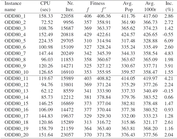
6.3.3. Results . . . 130
6.4. Application to the planning of maintenance tasks . . . 132
6.4.1. SNCF maintenance problem . . . 133
6.4.2. Uncertainties of an operational factory . . . 134
6.4.3. A robust schedule . . . 135
6.4.3.1. Variations of the unexpected factors . . . 137
6.5. Conclusions and perspectives . . . 139
6.6. Bibliography . . . 140
Chapter 7. Metaheuristics and Performance Evaluation Models for the Stochastic Permutation Flow-Shop Scheduling Problem . . . 143
Michel GOURGAND, Nathalie GRANGEONand Sylvie NORRE 7.1. Problem presentation . . . 144
7.2. Performance evaluation problem . . . 147
7.2.1. Markovian analysis . . . 147
7.2.2. Monte Carlo simulation . . . 153
7.3. Scheduling problem . . . 155
7.3.1. Comparison of two schedules . . . 156
7.3.2. Stochastic descent for the minimization in expectation . . . 157
7.3.3. Inhomogenous simulated annealing for the minimization in expectation . . . 157
7.3.4. Kangaroo algorithm for the minimization in expectation . . . 159
7.3.5. Neighboring systems . . . 161
7.4. Computational experiment . . . 161
7.4.1. Exponential distribution . . . 162
7.4.2. Uniform distribution function . . . 164
7.4.3. Normal distribution function . . . 167
7.5. Conclusion . . . 167
Contents 9
Chapter 8. Resource Allocation for the Construction of Robust Project
Schedules . . . 171
Christian ARTIGUES, Roel LEUSand Willy HERROELEN 8.1. Introduction . . . 171
8.2. Resource allocation and resource flows . . . 173
8.2.1. Definitions and notation . . . 173
8.2.2. Resource flow networks . . . 174
8.2.3. A greedy method for obtaining a feasible flow . . . 176
8.2.4. Reactions to disruptions . . . 176
8.3. A branch-and-bound procedure for resource allocation . . . 178
8.3.1. Activity duration disruptions and stability . . . 178
8.3.2. Problem statement and branching scheme . . . 179
8.3.3. Details of the branch-and-bound algorithm . . . 180
8.3.4. Testing for the existence of a feasible flow . . . 182
8.3.5. Branching rules . . . 183
8.3.6. Computational experiments . . . 184
8.3.6.1. Experimental setup . . . 184
8.3.6.2. Branching schemes . . . 185
8.3.6.3. Comparison with the greedy heuristic . . . 187
8.4. A polynomial algorithm for activity insertion . . . 187
8.4.1. Insertion problem formulation . . . 188
8.4.2. Evaluation of a feasible insertion . . . 189
8.4.3. Insertion feasibility conditions . . . 190
8.4.4. Sufficient insertions and insertion cuts . . . 191
8.4.5. Insertion dominance conditions . . . 192
8.4.6. An algorithm for enumerating dominant sufficient insertions . . . 193
8.4.7. Experimental results . . . 193
8.5. Conclusion . . . 194
8.6. Bibliography . . . 195
Chapter 9. Constraint-based Approaches for Robust Scheduling . . . 199
Cyril BRIAND, Marie-José HUGUET, Hoang Trung LAand Pierre LOPEZ 9.1. Introduction . . . 199
9.2. Necessary/sufficient/dominant conditions and partial orders . . . 200
9.3. Interval structures, tops, bases and pyramids . . . 201
9.4. Necessary conditions for a generic approach to robust scheduling . . . 202
9.4.1. Introduction . . . 202
9.4.2. Scheduling problems under consideration . . . 204
9.4.3. Necessary feasibility conditions . . . 205
9.4.4. Propagation mechanisms . . . 206
9.4.4.1. Time constraint propagation . . . 206
9.4.5. Interval structures for propagation . . . 208
9.4.5.1. Rank-interval based structures . . . 208
9.4.5.2. Task-interval based structures . . . 210
9.4.6. Discussion . . . 212
9.5. Using dominance conditions or sufficient conditions . . . 213
9.5.1. The single machine scheduling problem . . . 213
9.5.2. The two-machine flow-shop problem . . . 217
9.5.3. Future prospects . . . 221
9.6. Conclusion . . . 222
9.7. Bibliography . . . 222
Chapter 10. Scheduling Operation Groups: A Multicriteria Approach to Provide Sequential Flexibility . . . 227
Carl ESSWEIN, Jean-Charles BILLAUTand Christian ARTIGUES 10.1. Introduction . . . 227
10.2. Groups of permutable operations . . . 228
10.2.1. History, principles and definitions . . . 228
10.2.2. Representation and evaluation . . . 230
10.2.2.1. Earliest start time computation . . . 232
10.2.2.2. Latest completion time computation . . . 234
10.2.2.3. Quality of a group schedule . . . 234
10.3. The ORABAIDapproach . . . 235
10.3.1. The proactive phase: searching for a feasible and acceptable group schedule . . . 235
10.3.1.1. Construction of a feasible group schedule . . . 236
10.3.1.2. Searching for acceptability of the group schedule . . . 237
10.3.1.3. Increasing the group schedule flexibility . . . 237
10.3.2. The reactive phase: real-time decision aid . . . 237
10.3.3. Some conclusions about ORABAID . . . 238
10.4. AMORFE, a multicriteria approach . . . 238
10.4.1. Flexibility evaluation of a group schedule . . . 239
10.4.2. Evaluation of the quality of a group schedule . . . 240
10.4.3. Some considerations about the objective function definition . . . 241
10.4.4. Quality guarantee in the best case . . . 243
10.4.4.1. Advantages . . . 243
10.4.4.2. Respect for quality in the best case . . . 243
10.5. Application to several scheduling problems . . . 244
10.6. Conclusion . . . 246
10.7. Bibliography . . . 246
Chapter 11. A Flexible Proactive-Reactive Approach: The Case of an Assembly Workshop . . . 249
Contents 11
11.2. Definition of the control model . . . 251
11.2.1. Definition of the problem and its environment . . . 251
11.2.2. Definition of a solution to the problem . . . 251
11.2.3. Definition of the solution quality . . . 252
11.2.3.1. Preliminary example . . . 252
11.2.3.2. Performance of a solution . . . 253
11.2.3.3. Flexibility of a solution . . . 255
11.3. Proactive algorithm . . . 256
11.3.1. General schema of the proposed genetic algorithm . . . 256
11.3.2. Selection and strategy of reproduction . . . 258
11.3.3. Coding of a solution . . . 258
11.3.4. Crossover operator . . . 258
11.3.5. Mutation operator . . . 259
11.4. Reactive algorithm . . . 260
11.4.1. Functions of the reactive algorithm . . . 260
11.4.2. Reactive algorithms in the absence of disruptions . . . 261
11.4.2.1.A posterioriquality measures . . . 261
11.4.2.2. Proposed algorithms . . . 263
11.4.3. Reactive algorithm with disruptions . . . 264
11.5. Experiments and validation . . . 264
11.6. Extensions and conclusions . . . 265
11.7. Bibliography . . . 266
Chapter 12. Stabilization for Parallel Applications . . . 269
Amine MAHJOUB, Jonathan E. PECEROSÁNCHEZand Denis TRYSTRAM 12.1. Introduction . . . 270
12.2. Parallel systems and scheduling . . . 270
12.2.1. Actual parallel systems . . . 270
12.2.2. Definitions and notations . . . 271
12.2.3. Motivating example . . . 273
12.3. Overview of different existing approaches . . . 275
12.4. The stabilization approach . . . 276
12.4.1. Stabilization in processing computing . . . 276
12.4.2. Example . . . 278
12.4.3. Stabilization process . . . 280
12.5. Two directions for stabilization . . . 280
12.5.1. The PRCP∗algorithm . . . 281
12.5.2. Strong stabilization . . . 283
12.6. An intrinsically stable algorithm . . . 286
12.6.1. Convex clustering . . . 286
12.6.2. Stability analysis of convex clustering . . . 290
12.7.2. Influence of the initial schedule in the stabilization process . . . 295
12.7.3. Comparison of the schedules with and without stabilization . . . 297
12.7.4. Test 1 – comparison for Winkler graphs . . . 297
12.7.5. Test 2 – comparison for layer graphs . . . 298
12.8. Conclusion . . . 299
12.9. Bibliography . . . 300
Chapter 13. Contribution to a Proactive/Reactive Control of Time Critical Systems . . . 303
Pascal AYGALINC, Soizick CALVEZand Patrice BONHOMME 13.1. Introduction . . . 303
13.2. Static problem definition . . . 305
13.2.1. Autonomous Petri nets (APN) . . . 306
13.2.2. p-time PNs . . . 307
13.3. Step 1: computing a feasible sequencing family . . . 311
13.4. Step 2: dynamic phase . . . 317
13.4.1. Temporal flexibility . . . 317
13.4.2. Temporal flexibility and sequential flexibility . . . 319
13.4.2.1. Partial order in performance evaluation . . . 320
13.4.2.2. Partial order in proactive/reactive control . . . 322
13.5. Restrictions due to p-time PNs . . . 323
13.6. Bibliography . . . 325
Chapter 14. Small Perturbations on Some NP-Complete Scheduling Problems . . . 327
Christophe PICOULEAU 14.1. Introduction . . . 327
14.2. Problem definitions . . . 328
14.2.1. Sequencing with release times and deadlines . . . 328
14.2.2. Multiprocessor scheduling . . . 329
14.2.3. Unit execution times scheduling . . . 330
14.2.4. Scheduling unit execution times with unit communication times 331 14.3. NP-completeness results . . . 332
14.4. Conclusion . . . 340
14.5. Bibliography . . . 340
List of Authors . . . 341
Preface
This book is about scheduling under uncertainties. However, the problems concern the whole domain of decision aid. Of course, the question of decision aid under unexpected events or uncertainties is not new, but a recent awareness has come on the necessity to define specific models. This awareness has lead to research activities in various domains like location, communication or transportation network design, supply chain management, industrial planing and – of course – scheduling problems.
In Spring 2000, some members of the “GOThA” group (a French working group on “Theoretical scheduling and applications”) decided to create a sub-group working in the field of “flexibility”. It seemed convenient to gather the persons interested by the question: “how do we schedule under uncertainties?”. The success of this initiative was a surprise for their promoters themselves. In France only, among ten research teams were working on this problem. These teams wanted to communicate ideas, to unify the terminology, to exchange references. After multiple meetings during 2003, this group became a project “Scheduling with flexibility and robustness” among an official structure, the GDR-CNRS on Operations Research. The book Flexibilité et Robustesse en Ordonnancementpublished by Hermes in 2005 was the first conclusion of this project. This book is a revised version of this title.
Chapters 3 to 8 (5 to 8 with probabilistic hypotheses) consider that all the decisions have been taken before starting the schedule. In the approach of Chapters 9 to 13 most of the decisions are taken during the execution of the schedule. The last chapter considers on-line re-optimization.
Scheduling theory concerns several fields. Chapters 3, 5, 7, 10, 11 and 13 consider shop scheduling problems, whereas Chapters 6 and 8 consider project scheduling problems and Chapters 4 and 12 consider parallel computing. Chapters 9 and 14 do not consider a particular application field. But frontiers are sometimes thin.
We are very happy with this English version and hope that it will interest numerous researchers and scheduling practitioners.
Chapter 1
Introduction to Flexibility and
Robustness in Scheduling
1.1. Scheduling problems
A large variety of scheduling problems are to be found in many domains. Almost every sector is concerned by scheduling problems in the broad sense:
– Industrial production systems: problems may need to be solved simultaneously in machine scheduling and vehicle dispatching (automated guided systems, robotic cells, hoist scheduling problems), in workshop layout problems or supply chain management problems.
– Computer systems: for example, to make full use of the processing power provided by parallel machines or when scheduling tasks with resource constraints in real-time environments.
– Administrative systems: appointment scheduling in health care sector, general resource assignment, timetabling, etc.
– Transportation systems: vehicle routing problems, traveling salesman problems, etc.
In all cases, for a realization being described as a series of interdependent tasks, it is necessary to coordinate the implementation of these tasks, i.e. to allocate resources
Chapter written by Jean-Charles BILLAUT, Aziz MOUKRIMand Eric SANLAVILLE.
Flexibility and Robustness in Scheduling
zyxwvutsrqponmlkjihgfedcbaZYXWVUTSRQPONMLKJIHGFEDCBA
Edited by Jean-Charles Billaut, Aziz Moukrim
zyxwvutsrqponmlkjihgfedcbaZYXWVUTSRQPONMLKJIHGFEDCBA
& Eric Sanlavilleto tasks and set their execution dates. Sometimes a schedule simply consists of a sequence of tasks by machine, coupled with a simple rule for calculating task start times (for example earliest schedules). However, in the more general case it is necessary to allocate a start time to each task in the schedule definition.
The basic data of a scheduling problem (see for instance [BRU 07]) are: the tasks to schedule with their precedence constraints, their duration, resources that are necessary for their execution and a function to optimize.
Methods for solving scheduling problems draw from all the techniques of combinatorial optimization, whether approximate methods (greedy algorithms, local search, genetic algorithms, etc.) or exact methods (mathematical programming, branch-and-bound methods, dynamic programming, decomposition methods, constraint programming, etc.). Solving a particular problem may require the use of modeling tools for complex systems (simulation, Petri nets, etc.), thus leading to the definition of matchings between these methods.
The scheduling problems addressed in this book are described according to the classification schemes proposed in [GRA 79]. The scheduling problems are specified using a classification in terms of three fields,α|β|γ where αspecifies the machine environment,βthe operation characteristics, andγthe criterion to optimize.
1.1.1. Machine environments
The majority of scheduling problems correspond to a number of fundamental theoretical models. We have to schedule a set of n tasks or n jobs. The machine environments are specified in the fieldαseparated into two subfieldsα1α2. Depending on the values ofα1, we may distinguish the following models:
– Single machine problems. Each task Tj of duration pj runs on a dedicated machine that cannot handle more than one task at a time. In that case the fieldα1 is absent andα2= 1.
– Parallel machine problems. The tasks are to be executed on machines in parallel, andpijdenotes the execution time ofTjon machineMi:
- Ifα1=P, the machines are identical:pij =pjfor any machineMi. - Ifα1=Q, the machines are uniform:pij =pj/siwheresiis the processing speed of machineMi.
Introduction to Flexibility and Robustness in Scheduling 17
– Shop problems. In this model, a shop consists of m different machines. We consider a set of jobs that need to be performed. Each jobJj is described bynjtasks (which are calledoperations). OperationJj running on machineMiis denotedOij, and its duration is pij. Operations belonging to the same job cannot be carried out simultaneously. There are three main types of shop:
- Flow-shop. Each job consists ofmoperations and the order of execution on different machines is the same for each job. In this caseα1=F.
- Job-shop. The number of operations is not necessarily the same for each job, and every job has its own order of execution on the machines. In this caseα1=J.
- Open shop. This is the least constrained shop scheduling problem. The number of operations is not necessarily the same for each job, and the order of execution on the machines is completely free. In this caseα1=O.
– Project scheduling under resource constraints. In this model, known as the “resource constrained project scheduling problem” (RCPSP), we consider a set of tasks or activities. The execution of each taskTj requires the use of a fixed amount Rij of resourcei. The maximum capacity of each resourceiis available. The field α1takes the valuePS(“Project Scheduling”). Note that the case where the capacity is unlimited corresponds to the central problem in the well-known PERT scheduling model.
Ifα2is a positive integer, the number of machines or resources is assumed to be constant. If the fieldα2is absent then this number is assumed to be arbitrary.
1.1.2. Characteristics of tasks
The fieldβ=β1β2β3β4describes the task characteristics.
Preemption means that the execution of an operation or a task can be interrupted and completed later, either on the same machine or on another machine. An operation or task can be interrupted several times. If preemption is allowed thenβ1 = pmtn, otherwise fieldβ1is missing.
performed on two different processors (or machines),cjkcorresponds to the shortest delay between the end ofTjand the beginning ofTk, otherwise this delay is zero.
The release dates of tasks (earliest start times) are not necessarily identical. In this case,β3=rj. If all tasks are assumed to be available at time 0, the fieldβ3is missing.
Ifβ4=dj, we hope that the completion timeCjfor each taskTjwill be less than or equal todj, called thedue dateofTj. IfCjexceedsdj, the task is considered late.
1.1.3. Optimality criteria
When a schedule is fixed, the following variables can be computed for each task Tjor every jobJj:
– end date of the taskTjor jobJj, or completion time, notedCj; – latenessLj =Cj−djor tardinessTj = max{0, Cj−dj}; – unit penaltyUj= 0ifCj≤dj, otherwiseUj= 1;
– flow timeFj=Cj−rj.
Optimality criteria are functions to minimize. Usually, they integrate the above variables in the form of a maximum function or a sum function, possibly weighted. For example:
– the duration of the schedule ormakespanis the functionCmax= max1≤j≤nCj; – the weighted number of late tasks is the functionn
j=1wjUj.
Optimizing a single criterion is sometimes not sufficient, and in order to solve the problem, several conflicting criteria must be taken into account. For example, a company might want to minimize delivery delays and also to minimize its storage costs. These two criteria are clearly antagonistic, and multicriteria optimization methods are required to develop a procedure which will provide the best compromise solution [T’K 06].
We conclude this section by defining three scheduling classes:
– a schedule is said to besemi-activeif no task can be performed earlier without changing the order of execution or violating the constraints;
– a schedule is said to be active if no task can be performed earlier without violating the constraints;
Introduction to Flexibility and Robustness in Scheduling 19
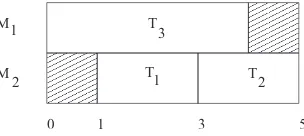
Figure 1.1 shows a single machine scheduling problem involving two tasksT1and T2 withp1 = 2,p2 = 1,r1 = 1andr2 = 0. The schedule shown in Figure 1.1a is semi-active but is neither active nor without delay, whereas the schedule shown in Figure 1.1b is semi-active, active and without delay.
b) a)
3 1
0 4
3 1
0
1 T 2 T 2
T 1
T
Figure 1.1.Examples of semi-active and delay-free schedules
Figure 1.2 shows a parallel machine scheduling (m= 2) of three tasksT1,T2and T3withp1 = 2,p2 = 2,p3 = 4,r1 = 1andr2 =r3 = 0. The schedule shown in Figure 1.2 is both active and semi-active but not without delay.
2 1
M M
3
2 T
5 T
3 1
0
1 T
Figure 1.2.An example of an active schedule that is not delay-free
1.2. Background to the study
The subject under consideration is scheduling and the problem addressed in this book is the integration of flexibility and robustness in scheduling problems.
Scheduling problems are widely discussed in the literature, in a large variety of contexts (see section 1.1). We distinguish here two major classes of approach:
common in the literature devoted to scheduling problems, and there are many books dealing with the most classic problems (see for example [BLA 01, BRU 07, PIN 01]). – On-line methods. When the algorithm does not have access to all the data from the outset, we say that the data become available step by step, or “on-line”. Different models may be considered here. In some studies, the tasks that we have to schedule are listed, and appear one by one. The aim is to assign them to a resource and to specify a start time for them. In other studies, the duration of the tasks is not known in advance. These problems have given rise to many theoretical studies (e.g. [SGA 98, FIA 98]).
Flexibility occurs at the boundary between these two approaches: some information is available concerning the nature of the problem to be solved and concerning the data. Although this information is imperfect and not wholly reliable, it cannot be totally ignored. We also know that there will be discrepancies, for a number of reasons, between the initial plan and what is actually realized. Given that disruptions will occur and unforeseen circumstances arise, the aim is to propose one or more solutions that adapt well to disruptions, and then produce reactive decisions in order to ensure a smooth implementation. Another parameter here is the freedom left to the scheduler about the set of solutions it might be possible to propose: this flexibility is internal to the individual problem. Hence there are two kinds of flexibility, this internal flexibility, and thechosen flexibility, that the method really use when proposing a set of solutions (see section 1.4).
Robustness refers to the performance of an algorithm in the presence of uncertainties. Measures of robustness are required, which we will show later. Robustness can be defined at several levels: we can speak of the robustness of a solution of course, but also of the robustness of a procedure or of a conclusion [ROY 02]. Robustness is a qualifier which generally refers to a capacity to tolerate approximations (on the assumptions, model or data [ROY 02]). It is also a measure of the result after the application of a procedure in the presence of uncertainties, or after the appearance of uncertainty, for example relative to the operation duration the transport time, the availability of the most qualified personnel, etc. It is the performance characterization of an algorithm (or a complete process of schedule construction) in the presence of uncertainties (see section 1.5).
1.3. Uncertainty management
Introduction to Flexibility and Robustness in Scheduling 21
possible. We restrict ourselves to some basic works, leaving the more specialized studies in the bibliographies of the different chapters.
The book by Kouvelis and Yu [KOU 97] presents the sources of uncertainty in operations research, particularly in scheduling, and provides a discussion on models (see also the article by Daniels and Kouvelis [DAN 95]). The article by Davenport and Beck [DAV 00] is a very detailed review with a classification of possible approaches, while Herroelen and Leus [HER 05] focus on project scheduling and describe a wide range of methods.
1.3.1. Sources of uncertainty
The data associated with a scheduling problem are the processing times, occurrence dates of some events, some structural features, and the costs. None of this data is free from factors of uncertainty.
The duration of tasks depends on the conditions of their execution, in particular on the necessary human and material resources. They are thus inherently uncertain, regardless of contingent factors that may impair their execution. At any time, communications between two tasks depend on the state of the communication network, the level of contention, the availability of links, and so on. Similarly, transportation times for components between separate operations in a production process will depend on the characteristics of the transportation resources available. Finally, in a production context, some resources such as versatile machines require a reconfiguration time between operations. This time depends on the type of tools needed and the location of these tools in the shop, not to mention the operator carrying out the reconfiguration.
The start times for some events within a schedule can be part of the initial data. This is the case for the arrival of a task (release date), which often depends on events outside the studied system, such as events in the supply chain or a customer order. The same is true of the due date of a task. The periods of availability of human or machine resources is also difficult to predict precisely, due to maintenance, delays or unforeseen absences of an operator or a raw material.
Finally, if a cost is associated with a task, it can be changed without notice, especially when the considered system is part of a larger hierarchical system: the priorities are set at a higher level.
Thus, no data can be regarded as immutable, although the possibility of a change depends on the context. We can consider two cases for each piece of data (duration, date or cost): either its value is uncertain, that is to say it may take any value inside some fixed set; or its value may be subject to a disturbance, meaning that it is set in order to ensure normal functioning of the system, but can be changed by some unexpected event. This is of course always the case for structural data, which are modified according to contingent events.
1.3.2. Uncertainty of models
It follows from the above discussion that non-deterministic models are essential for solving concrete problems in scheduling, because of the inherent uncertainty in the data. Let us first consider the hypothesis of randomness which has given rise to a longstanding branch of research: stochastic scheduling. Here, all data (durations and also the dates of events, including possible disruptions) are modeled using random variables, and possibly constants. The probability of events is assumed to be known. From this stochastic model, it is theoretically possible to compute a priori the best schedules, or rather (in the case of possible disruptions) policies, i.e. the most successful decision sets (see the chapter by Weis [WEI 95] in [CHR 95] for a presentation of stochastic scheduling, as well as the book by Pinedo [PIN 01]).
This assumption of randomness is not always made, for at least three reasons. First,a prioriknowledge about the data is not always sufficient to deduce the laws of probability associated with it, especially if the problem is addressed for the first time. Secondly, assumptions regarding independence are rarely justified: a major source of disruptions may often result in a number of uncertainties concerning various data. Finally, even if a stochastic model can be envisaged, it is often too complex to be usable.
Introduction to Flexibility and Robustness in Scheduling 23
application of which to scheduling problems has seen some recent developments. This is not addressed in this book, but has been the subject of a book published by Hapke and Slowinski [SLO 00]; see also Duboiset al.[DUB 03].
It may happen that the data are outside the considered sets. One simple solution to this is not to propose a set at all. Nevertheless, a commonly-used technique is to assign to each piece of data a central value, its estimate, and all these estimated values may then be used while anticipating the possible differences at the execution step.
To sum up, the data can be represented as either random variables (stochastic model), real intervals (interval model) or discrete sets (scenario model). They may or may not be associated with an initial estimate. It is of course possible to combine different modes of representation!
1.3.3. Possible methods for problem solving
We now look at different methods for solving a scheduling problem with uncertainties. The choice depends of course on the chosen model. Let us first list the steps needed to solve such a problem.
1.3.3.1. Full solution process of a scheduling problem with uncertainties
Obtaining a complete solution to the problem requires the following steps: – Step 0: defining a static problem. The definition includes, in addition to the classical specifications in deterministic scheduling, the specifications of uncertainties and their modeling. The concept of schedule quality must also be specified at this stage.
– Step 1: computing a set of solutions, i.e. a family of feasible schedules achievable by a static algorithmα(static phase). A set of solutions can be obtained from a single solution, for example when the start times of some tasks may vary within a known interval.
– Step 2: during execution, a unique solution is calculated, that is to say the schedule actually carried out, which is the outcome of applying a dynamic algorithm δ(dynamic phase) to the set of possible solutions.
1.3.3.2. Proactive approach
In this approach, the focus is on step 1: knowledge of the uncertainties is used by the static algorithm to build one baseline schedule or a family of schedules. This family can be described either explicitly or implicitly. In the literature we also encounter the term predictive approach, the difference being that the schedule constructed in the latter case, using a static algorithm, does not take uncertainty into account. The starting point of this book is that it must be taken into account, and therefore we shall only look at proactive approaches.
In both approaches, predictive and proactive, step 2, during the execution, does not require any calculations: according to the real value of data, the baseline schedule is used or it is adjusted to remain feasible. These choices or adjustments are made using simple rules, such as waiting for a task to complete if it is overdue, or taking a particular action when a particular event occurs.
A stochastic model can give rise to a proactive approach, the uncertainty being taken into account in the computation of a baseline schedule.
1.3.3.3. Proactive/reactive approach
It is natural to couple a proactive approach, when it proposes a family of schedules, with a more elaborate step 2: as knowledge of the actual data values is acquired, and possibly after a disruption, a non-trivial dynamic algorithm is used to choose among the schedules selected in the previous (static) step those that prove to be the most efficient. This approach, responding to actual conditions while using the results of step 1, is called proactive/reactive.
In addition, let us note that it is often impossible to take all uncertainties into account, in particular disruptions, during the static phase. The example of machine failure is the most obvious but not the only one. The dynamic algorithm is then a necessity.
Introduction to Flexibility and Robustness in Scheduling 25
1.3.3.4. Reactive approach
In the purely reactive approach, the choices specifying a schedule are made during the dynamic phase. We must keep in mind that depending on the context, the reaction time required may vary from several days for some projects to less than a second for computer applications or embedded systems. If we have relatively accurate information regarding the value of data in the ongoing schedule (see step
0), the ideal scenario is to compute the optimal decision at every point where a
choice can be made, which corresponds to post-optimization, here used in an iterative manner. However, simple decision rules are more often applied, such as giving priority to tasks with smaller margins. These rules rarely build optimal schedules. In the particular case of stochastic models, it is sometimes possible to show that one set of rules (here called policy) is the best, for example according to the criterion expectation(see section 1.5).
Finally, when very few assumptions are made about the data (no estimates), decisions to be made at each moment are very difficult to evaluatea priori, which leads us into the area ofon-line schedulingmentioned earlier. A typical case is when the characteristics of a task (duration or mode of execution) are unknown until the job is ready to be executed. The on-line scheduling reviewed by Sgall [SGA 98] is beyond the scope of this book.
1.4. Flexibility
The introduction of flexibility into a scheduling problem reflects the degree of freedom during the implementation phase of the scheduling. This flexibility can take several forms:
– Time, ortemporalflexibility, i.e. regarding the starting times of operations. This flexibility can be seen as implicit in scheduling, since it allows some operations to drift over time, if conditions dictate. This is the first level of flexibility in scheduling.
– Flexibility regarding order of execution, or sequential flexibility. This means being able to change the order in which the operations should run on the machines, and implicitly presupposes temporal flexibility. It can be proposed during the execution of the sequence, allowing some operations to overtake others, if the conditions require it.
– Flexibility in the execution mode. The execution mode encompasses the possibility of preemption, overlap, changes in product range, whether set-up time is taken into account, changes in the number of resources required to perform an operation, and so on. This flexibility can be proposed depending on the context to overcome a difficult situation.
Flexibility, which is a degree of freedom available during the operational phase, can be harnessed in step 1, during the static phase. Indeed, some methods, in order to give more flexibility regarding start times, will allocate the available margins to operations in proportion to their length, for example, or will allocate margins to the operations considered as the most critical, as is the case with the concept of buffer in the critical chain [GOL 97, HER 01]. In order to give more sequential flexibility, the concepts of groups of swappable tasks ([ART 99, ART 05]) and of partial order between tasks [ALO 02, WU 99, MOU 99] have been proposed. These methods were designed to build robust schedules.
The challenge when introducing flexibility is finding a way of measuring the level of flexibility obtained. Some approaches rely on measuringa posteriorithe utility of the flexibility proposed by comparing the quality of a flexible solution to that of a non-flexible solution in the presence of disturbances. It is consequently the robustness measure that should indicate whether or not a particular flexible solution is better than a non-flexible solution.
1.5. Robustness
It is really difficult to give a unique definition for robustness, as this concept is differently defined in several domains. Furthermore, often in the literature, the definition often remains implicit in the literature or is determined by the specific target application. Finally, most authors prefer to use the concept of robust solution (and here, of robust schedule).
Let us first propose some consensus definition: a schedule is robust if its performance is rather insensitive to the data uncertainties. Performance must be understood here in the broad sense of solution quality for the person in charge; this naturally encompasses this solution value relatively to a given criterion, but also the structure itself of the proposed solution. The robustness of a schedule is a way to characterize its performance.
Introduction to Flexibility and Robustness in Scheduling 27
solutions according to the real problem data. Throughout this section, the termmethod will be used to designate the whole building process of the final schedule. Thus, we follow Bernard Roy [ROY 02] who states that the person in charge is not interested in a specific solution, but in the set of solutions a method can build according to the real data, and by their variability. The questions raised in this work, in the larger framework of decision aid are fundamental also for scheduling under uncertainties. When the whole method is not explicit, but one stage alone (static or dynamic) is under study, it is then legitimate to use the terms of robust algorithm, or even of robust schedule.
The curious reader might also find it very useful to look for works about robust optimization at large, reflecting the diversity of the approaches; see Kouvelis and Yu [KOU 97], Ben-tal and Nemirovski [BEN 99], Aïssiet al.[AÏS 07], among many others.
In order to characterize robustness, different tools that might be used are presented. This in fact implies that several types of robustness exist. The following notations shall be used:
–P: a static problem, together with uncertainties description. HenceP is a set, possibly infinite, of instances of the deterministic problem.
–I: an effective instance of P (describing the effective conditions met during execution) also called the scenario.
–S: an effective schedule, obtained by the studied building process. S varies according to the considered scenario and in cares of possible ambiguity it is noted SI.
–zI(S): performance of scheduleS realized onI, simply denotedzIif there is no ambiguity.
–z∗
I: performance of an optimal schedule onI.
In deterministic scheduling, the performance criterion is fixed from the beginning, and it is immediately computable for a fixed schedule. In scheduling with uncertainties, there are several possible measures for a given criterion, and we try to give below a typology of these measures.
1.5.1. Flexibility as a robustness indicator
be tempted to report any decision at execution phase (reactive approach); this is not always the best for the quality of the final solutions (myopic behavior, temporal constraints). Another key feature of a method is its feasibility for all considered uncertainties. If uncertainty is large, and/or disturbances numerous, the feasibility cannot be guaranteed in general (unless some exceptional repair mechanism can be set). Hence we should always try to maximize the method flexibility, expressed as its feasibility for the largest set of scenarios (here understood in a broad sense). It must be noted that starting from the internal or allowed flexibility, we consider now a chosen flexibility. In that sense, a flexibility indicator can rightly be considered as a robustness measure for the method at hand; see Chapters 9 and 11 in this book.
Still, it is always a good idea to couple that indicator with another measure, bound to the performance in the classical sense. Concerning the studies from the literature, the feasibility guarantee is usually implicitly accepted as a property of the method (a hypothesis that should be justified). In that case, flexibility is not measured.
1.5.2. Schedule stability (solution robustness)
Here the performance criterion (makespan, mean flow-time, etc.) is not considered. For a given method, we try to minimize the differences between the different solutions obtained (by the same method) for different scenarios. In automation literature this specific aspect of robustness is sometimes called stability, a term that shall be used in that sense inside this book (see Chapters 8 and 13); ideally, there is one schedule unchanged for the different scenarios, hence it isstable. The difference between two schedules, denoted their distanced, can be for instance the number of permutations between tasks or machines, or any other adequate measure in the considered context. Then we might try to minimize either the largest distance between two solutions, or the largest distance with respect to some reference, or baseline, scheduleS. In the˜
second case, we speak naturally of the stability of this baseline schedule, or ofsolution robustness[HER 05].
R1= max
I,I′∈Pd
SI, S′ I
R′
1= max
I∈Pd
SI,S˜
Introduction to Flexibility and Robustness in Scheduling 29
1.5.3. Stability relatively to a performance criterion (quality robustness)
Again, we try to minimize a distance between the solutions obtained by different scenarios. This time though, the distance is measured with respect to the obtained value of the criterion. In [HER 05] this is called quality robustness, meaning that the quality (criterion value) of the baseline schedule should remain equivalent in all scenarios. With different models and points of view, such robustness measures are used in Chapters 6, 7, 12 and 14. If this value is considered as one characteristic, among others, of a schedule, it is a particular example of the previous case: we look for a set of solutions with close performances. Most often this approach is used jointly with a model based on estimations of the data (scenarioI˜). There is a baseline
schedule, and the robustness measure is given by the largest difference between the performance of this schedule for the initial scenariozI˜, and the performance obtained for any other scenario:
R2= max
I∈P zI zI˜
(relative difference)
R′
2= max
I∈P zI−zI˜
(absolute difference)
R2can be called thestability ratio. In one important case, only one schedule is built whatever the scenario (this implies the feasibility hypothesis). In fact, a family of schedules is usually considered, obtained from an initial schedule by accepting some amount of temporal flexibility. The robustness of this scheduleSis measured byR2 orR′2,zIbeing here the performance ofSforI.
From the perspective of the associated optimization problems, such as looking for the most robust process forR2, the problem is equivalent to minimizing the largest value of the criterion on the set of possible scenarios as soon aszI˜is fixed.
When statistical data are available, a stochastic model can be used and it is possible to look for schedules whose mean behavior is good. Although the robustness measures are obtained fromR2 or R′2 by replacing the maximum by, for instance, the expectation, it is less natural to speak of stability (except that it means some guarantees can be obtained about, for instance, the mean behavior). The obtained measures are here the traditional measures in stochastic optimization, particularly:
R3=EI∈P
zI (criterion expectation)
set of solution, or a set with good mean behavior. That is why many authors keep the term robustness for other measures.
1.5.4. Respect of afixed performance threshold
Frequently, a target performance z˜ is defined a priori. The method is then considered as robust if no performance schedule exceeds this threshold, whatever the scenario. Hence the measure
R4= max
I∈P
zI−z˜
(absolute deviation with respect to some threshold)
Of course, the associated optimization problem is the same as for the stability with respect to the performance criterion (see section 1.5.3) and the same drawback holds.
In the case of a stochastic model, it is logical (see Daniels and Carillo [DAN 97]) to minimize the probability of exceeding the threshold:
R5=PI∈PzI≥z˜ (service level measure)
The difficulty in using this measure (see Chapter 5) comes from the fact that we must know the probability law associated with the random variablez.
1.5.5. Deviation measures with respect to the optimum
Robustness is measured here by comparing the criterion value obtained by the method and the optimum value, this for all scenarios. Following [DAN 95, KOU 97] we use the term of deviation: absolute deviation if the difference is computed; relative deviation for the ratio. There are several possibilities for using these deviations. One possibility is to compute their maxima, or their expectation in a stochastic setting. Thus, two relative measures are possible:
R6= max
I∈P zI z∗ I
(worst case relative deviation)
R7=EI∈P zI
z∗ I
(relative deviation in expectation)
and the corresponding absolute measuresR′
Introduction to Flexibility and Robustness in Scheduling 31
Computing these measures supposes that the optimal solution can be computed for each scenario, and in the stochastic case, that the probability of each scenario is known. This is not always possible, and we might just compute some upper bound, called thesensitivity bound, absolute or relative (see Chapter 4). It is also possible in the stochastic case to compute an approximation ofR7orR′7, by computing a mean after sampling the scenarios, see Kouvelis et al.[KOU 00] and more generally the stochastic optimization literature. We might speak then ofsampled mean deviation.
1.5.6. Sensitivity and robustness
In the literature, it is sometimes difficult to separate sensitivity analysis and robustness. In fact the sensitivity analysis tries to answer the “what if...” questions. It deals with disturbances more than with general uncertainty: data are fixed but might be disturbed, a baseline schedule S˜ is given, which is most often optimal.
Sensitivity analysis tries to measure the performance degradation ofS˜for a particular
disturbance. It is not concerned with the execution phase: the robustness of a static algorithm is measured. Among the above measures, sensitivity analysis might use R1,′ R
2,R6orR′6, and does not deal with probabilistic models. Furthermore, it comes historically from linear programming (LP), and as for LP disturbances concerns one parameter at a time. In LP, the maximum change of a parameter for which the current basis is still optimal is easy to compute. In scheduling, Sotskovet al.[SOT 98] did introduce the stability radiusρS˜. Computing the radius is equivalent to searching for the maximum disturbance size for whichR′
2= 0. Hall and Posner [HAL 04] present a classification and many results about sensitivity analysis in scheduling.
It is of course possible to extend the analysis to a true uncertainty on data simultaneously considered (see [PEN 01] and Chapters 3 and 4 in this book), if the study is restricted to the static phase and to some disturbance types (taking into account the breakdowns, for instance, seems impossible). However, it is then difficult to show results on the stability radius for instance.
1.6. Bibliography
[AÏS 07] AÏSSI H., BAZGAN C. and VANDERPOOTEN D., “Min-max and min-max regret versions of some combinatorial optimization problems: a survey”, p. 1–32, Annales du Lamsade. ROYB., ALOULOUM.A. and KALAIR. (Eds.):Robustness in OR-DA, Paris, 2007.
[ART 99] ARTIGUES C., ROUBELLAT F. and BILLAUT J.-C., “Characterization of a set of schedules in a resource-constrained multi-project scheduling problem with multiple modes”,International Journal of Industrial Engineering, vol. 6, no. 2, p. 112–122, 1999.
[ART 05] ARTIGUES C., BILLAUT J.-C. and ESSWEIN C., “Maximization of solution flexibility for robust shop scheduling”,European Journal of Operational Research, vol. 165, no. 2, p. 314–328, 2005.
[AVE 00] AVERBAKH I., “On the complexity of a class of combinatorial optimization problems with uncertainty”,Mathematical Programming, vol. Ser A 90, p. 263–272, 2000.
[BEN 99] BEN-TAL A. and NEMIROVSKI A., “Robust solutions of uncertain linear programs”,Operations Research Letters, vol. 25, p. 1–13, 1999.
[BLA 01] BLAZEWICZ J., ECKER K.H., PESCH E., SCHMIDT G. and WEGLARZ J., Scheduling Computer and Manufacturing Processes, Springer-Verlag, Berlin, 2nd edition, 2001.
[BRU 07] BRUCKERP.,Scheduling Algorithms, Springer-Verlag, Berlin, 5th edition, 2007. [CHR 95] CHRÉTIENNE P., COFFMAN JR. E.G., LENSTRA J.K. and LIU Z. (Eds.),
Scheduling Theory and its Applications, John Wiley & Sons, 1995.
[DAN 95] DANIELSR.L. and KOUVELISP., “Robust scheduling to hedge against processing time uncertainty in single stage production”, Management Science, vol. 41, no. 2, p. 363–376, 1995.
[DAN 97] DANIELS R.L. and CARILLO J.E., “β-robust scheduling for single-machine systems with uncertain processing times”,IIE Transactions, vol. 29, p. 977–985, 1997.
[DAV 00] DAVENPORT A.J. and BECK J.C., A survey of techniques for scheduling with uncertainty, available in http://www.eil.utoronto.ca/profiles/chris/chris.papers.html, 2000.
[DUB 03] DUBOIS D., FARGIER H. and FORTEMPS B., “Fuzzy scheduling: modelling flexible constraints vs coping with incomplete knowledge”, European Journal of Operational Research, vol. 147, p. 231–252, 2003.
[FIA 98] FIAT A. and WOEGINGERG.J. (Eds.), Online Algorithms, The State of the Art, Lecture Notes in Computer Science, Springer, 1998.
[GOL 97] GOLDRATTE.M.,Critical Chain, The North River Press Publishing Corporation, Great Barrington, 1997.
[GRA 79] GRAHAM R.E., LAWLER E.L., LENSTRA J.K. and RINNOOY KAN A., “Optimization and approximation in deterministic sequencing and scheduling: a survey”, Ann. Discrete Math., vol. 4, p. 287–326, 1979.
Introduction to Flexibility and Robustness in Scheduling 33
[HER 01] HERROELEN W. and LEUS R., “On the merits and pitfalls of critical chain scheduling”,Journal of Operations Management, vol. 19, no. 5, p. 559–577, 2001.
[HER 05] HERROELENW. and LEUSR., “Project scheduling under uncertainty, survey and research potential”,European Journal of Operational Research, vol. 165, p. 289–306, 2005.
[KOU 97] KOUVELIS P. and YU G., Robust Discrete Optimisation and its Applications, Kluwer Academic Publishers, 1997.
[KOU 00] KOUVELIS P., DANIELS R.L. and VAIRAKTARAKIS G., “Robust scheduling of a two-machine flow shop with uncertain processing times”, IIE Transactions, vol. 32, p. 421–432, 2000.
[MOU 99] MOUKRIM A., SANLAVILLE E. and GUINAND R., “Scheduling with Communication Delays and On-line Disturbances”, in AMESTOYP. (Ed.),Euro-Par’99, Toulouse, France, LNCS 1685, p. 350–357, 1999.
[MUL 95] MULVEYJ.M., VANDERBEIR.J. and ZENIOSS.A., “Robust optimization of large scale systems”,Operations Research, vol. 43, p. 264–281, 1995.
[PEN 01] PENZ B., RAPINE C. and TRYSTRAM D., “Sensitivity analysis of scheduling algorithms”,European Journal of Operational Research, vol. 134, p. 606–615, 2001.
[PIN 01] PINEDOM.,Scheduling: Theory, Algorithms, and Systems, Prentice Hall, Englewood Cliffs, 2nd edition, 2001.
[ROY 02] ROYB., “Robustesse de quoi et vis-à-vis de quoi mais aussi robustesse pourquoi en aide à la d´cision?”,Newsletter of the European Working group “Multicriteria Aid for Decisions”, vol. 3, no. 6, p. 1–6, 2002.
[SGA 98] SGALLJ., “On-line scheduling – a survey”, p. 196–231, in Fiat and Woeginger (Eds.) [FIA 98].
[SLO 00] SLOWINSKI R. and HAPKE M., Scheduling Under Fuzzyness, Physica-Verlag, Heidelberg, 2000.
[SOT 98] SOTSKOV Y.N., WAGELMANS A. and WERNER F., “On the calculation of the stability radius of an optimal or an approximate schedule”,Annals of Operational Research, vol. 83, p. 213–225, 1998.
[T’K 06] T’KINDT V. and BILLAUT J.-C.,Multicriteria scheduling, Springer, Berlin, 2nd edition, 2006.
[WEI 95] WEISS G., “A tutorial in stochastic scheduling”, p. 33–64, in Chrétienne et al. [CHR 95].
Chapter 2
Robustness in Operations Research
and Decision Aiding
It is always advisable to perceive clearly our ignorance.
(Charles Darwin)
2.1. Overview
The search for robustness is an ever present concern is Operations Research and Decision Aiding (OR-DA) where increasingly rich and diversified methodologies and concepts are emerging. The term “robust” applies to a large variety of objects such as solution, method and conclusion. In OR-DA, the notion of robustness is often used in the same way as (sometimes even instead of) flexibility, stability, sensitivity and even equity in certain cases.
Faced with this diversity, I think it is necessary to highlight what seems to be the generally used meaning for the term “robust” in OR-DA (section 2.1.1) before specifying the reasons leading to the concern for robustness in this discipline (section 2.1.2) and presenting the structure of this chapter (section 2.1.3).
Chapter written by Bernard ROY.
Flexibility and Robustness in Scheduling
zyxwvutsrqponmlkjihgfedcbaZYXWVUTSRQPONMLKJIHGFEDCBA
Edited by Jean-Charles Billaut, Aziz Moukrim
zyxwvutsrqponmlkjihgfedcbaZYXWVUTSRQPONMLKJIHGFEDCBA
& Eric Sanlaville36 Flexibility and Robustness in Scheduling
2.1.1. Robust in OR-DA with meaning?
As I see it, robust is a term that is generally used in the sense of a capacity for withstanding “vague approximations” and/or “zones of ignorance” in order to prevent undesirable impacts, notably the degradation of the properties to be maintained.
“Vague approximations” can refer to a way of modeling, the restrictive character of certain hypotheses, mode of value allocation to data and/or parameters, etc.
“Zones of ignorance” may deal with the complexity of certain phenomena and of value systems but mostly the future: trends, contingencies, behavior of others, etc.
Here are a few examples to illustrate this meaning of the term “robust” in scheduling. In Chapter 1, a solution is said to be robust if its “performance is rather insensitive to data uncertainties and disturbances”. In this context, insensitivity to data uncertainty means resisting to this uncertainty1. The uncertainty in question can
for example refer to the way of modeling which processes certain data as insignificant or not influenced by contingencies, a Gaussian hypothesis simplifying the mode of consideration of a random phenomenon or the approximate character of values attributed to data (processing time, due date, etc.).
In some maintenance studies, scheduling must be conceived to guarantee deadlines are respected even though the jobs to be done are not well known (resistance to a certain form of ignorance). Job-shop scheduling may have to be chosen for its capacity to face an order book that is only partially known or with unknown reactions to delays that the end customer may encounter because of contingencies. Climate conditions, as well as work-related accidents or social upheavals, are sources of ignorance that project management may have to consider.
Two comments seem necessary to specify the meaning of what was just discussed: 1) Even though the borderline between vague approximations and zones of ignoranceis far from being well defined, all vague approximations do not come from
a zone of ignorance and all zones of ignorance do not lead to vague approximations.
2) Resistance can have the following meanings: protecting from, adapting to, being rather insensitive to, remaining stable, settling a certain form of equity, etc.
We will now examine the reasons resulting in the need to resist these vague approximations and zones of ignorance in OR-DA.
2.1.2. Why the concern for robustness?
In OR-DA, the capacity for resistance qualified by robustness is required in order to be protected from undesirable impacts, impacts that should be apprehended taking into account these vague approximations and/or zones of ignorance that need to be resisted. The nature of these impacts, along with the (very often subjective) way of assessing their undesirable character, are contingent to the context involved. The concerns motivating the search for robustness are extremely diversified for these reasons. I will settle for illustrating them through a series of examples in this chapter:
i) Exceptional character decisions
– Layout of a large linear infrastructure (very high speed train line, highway, high-tension line, etc.): throughout the execution (five years or more), what reactions will it generate? Once this is finished, what standards will it be judged by? Will the size be adapted to traffic?
– Construction of a sanitation or waterworks system: knowing that implementing such activities, as with the evolution of consumption patterns, can only be defined in large variation ranges, will the designed system be able to fulfill population requirements in the planned horizon without needing adjustments leading to prohibitive costs?
– Updating of equipment: considering the evolution of technology and environmental standards, when should the decision be made to update?
ii) Sequential character decisions
– Plan designed to be implemented in stages: how will the contexts in future stages be affected by the decisions taken at this present stage? Do they allow for possible evolutions of these contexts by keeping the range of adaptations and reactions open?
38 Flexibility and Robustness in Scheduling
iii) Choice of a method for repetitive applications
– Management support method for restocking a store: does the method protect against out of stock risks that could result from a failure to respect of delivery lead times by suppliers? Is it adapted for possible evolutions of purchase agreements?
– Method controlling budget distribution between members in a group: knowing that the size and composition of beneficiary groups can greatly change over time and space, will the method retained be considered fair in all cases where it will be applied? – Adjustment method for a model dedicated to emphasizing the way in which different factors contribute to global client satisfaction during consecutive surveys: how can we avoid the results depending on final retained values (chosen in a relatively arbitrary manner in certain intervals) for different technical parameters involved in the model?
2.1.3. Plan of the chapter
In the next section, I will examine where, for a decision aiding problem (DAP), “vague approximations” and “zones of ignorance” come from, for which the need for protection leads to the search for robustness. These vague approximations and zones of ignorance are closely linked to the way that the decision aiding problem is formulated (DAPF). They can also depend (although generally less so) on the
processing procedure applied to this formulation in the decision aiding process. This leads me to introduce the general concept of version. In section 2.3, I will specify
the meaning I give to several currently used terms (procedure and method notably) in order to clarify their links with the concern for robustness. In section 2.4, I will focus on the way to take robustness into consideration: what must be robust? How can we formalize robustness? In what form can vague approximations and zones of ignorance be taken into account? Unfortunately, many questions raised here will remain unanswered. A brief conclusion will complete this chapter.
2.2. Where do “vague approximations” and “zones of ignorance” come from? – the concept of version
2.2.1. Sources of inaccurate determination, uncertainty and imprecision
studied, the way it is formulated and the process mode applied. Nevertheless, I think it is possible to see them whatever they are as frailty pointsconnected to sources of inaccurate determination, uncertainty or arbitrariness(see [ROY 89]). The vague
approximations and zones of ignorance that must be resisted actually come from such sources. They can, it seems, be classified into three categories (even though the line separating these categories is not perfectly well defined, they affect sides of the DAPF which I think it is important to distinguish):
– SourceS ·α: vague, uncertain, unknown, and even undetermined character of factual data, objective descriptions of phenomena and purely technical procedural aspects in relation to the form in which they must occur during the aiding process in the present situation.
This source may, for example, affect frailty points such as: processing times, due dates, process cost, failure probabilities, probability distributions chosen for modeling a random factor, discrimination thresholds, values given to the parameters playing a mostly technical role in a model or procedure, techniques used to adjust a model intended to represent complex phenomena, etc.
– SourceS·β: implementation conditions of the decision that must be taken; these
conditions can be influenced by the future state of the environment:
- during implementation if the decision is punctual (i.e., taken all at once); - by consecutive environmental steps if the decision is sequential.
This source may, for example, affect frailty points such as: what will have happened (during implementation), labor and/or raw material cost, interest rates, consumption patterns, boundaries of what is acceptable (social and environmental standards among others) or the presence or absence of disrupting events (unavailable personnel or equipment, opposition of some stakeholders, climatic incidents, etc.).
– SourceS·γ: eminently subjective character of different aspects (not dealing with
sourcesS·αandS·β) dealing with feasibility, relative interest and process modes of
the different potential actions, especially the fuzzy, unstable and possibly incoherent and/or incomplete character of value systems which are supposed to prevail in the decision aiding process.
40 Flexibility and Robustness in Scheduling
scale, the way to apprehend attitude toward risk, the place reserved for certain actors (notably future generations).
2.2.2. DAP formulation: the concept of version
The expression DAP formulation must be taken in a very general sense. It
obviously includes the model, insofar as there is modeling (see section 2.3.3 below), but in a broader sense, everything that was in question and has finally been retained to contain and consequentlyformulate the problem, including the problematic (the way
in which decision aiding was conceived, see [ROY 96], Chapter 6), the properties to preserve and, in general, the undesirable impacts from which we want to be protected.
When we start being concerned about robustness in OR-DA, it is necessary in my opinion to start by identifying in DAPF what I have called frailty points connected to each of the three types of sourcesS·α,S·β,S·γ. Relative to each
of these frailty points, we should then explain the different options which deserve
to be considered within this formulation in order to take inaccurate determination, uncertainty and arbitrariness margins into consideration from these sources. The selection of a specific option for each of the identified frailty points defines what I proposed (see [ROY 02, ROY 07]) to call aversionof DAPF. If it is carried out without
precautions, this selection can very well lead to combinations lacking in coherence or plausibility. LetVˆ be the set of versionsV corresponding to combinations of options
deemed (possibly from very subjective bases) to be of interest (Vˆ cannot be discrete).
From this definition, two versions ofVˆ can notably differ by:
1) The values assigned to certain factual data or technical parameters characterizing events, phenomena, etc.: this is the case in particular with vague approximations and zones of ignorance fromS.α; when in the DAPF, this source is
the most significant, the wordversionbecomes synonymous withinstanceordatasets.
2) The way that we describe the future universe in which the decision must be executed: this is the case in particular with vague approximations and zones of ignorance fromS.β; when in the DAPF, this source is the most significant, the word
versionbecomes synonymous withscenario.
3) The way in which ambiguities, uncertainties and the multiplicity of value systems are taken into consideration: with vague approximations and zones of ignorance fromS.γ this is particularly the case for; when in the DAPF, this source
I think it is useful to emphasize that the way in which Vˆ versions distinguish
themselves does n