Shifts: Permanent and Temporary
Consequences of Intersectoral Shocks
Bruno Chiarini,Istituto Universitario Navale Di Napoli
Paolo Piselli, Banca D’Italia
The main purpose of this study is to examine the effect of allocative disturbances using Italian labour market data and a VECM (vector error correction model). In order to measure sectoral shifts in labour demand, we use Neumann-Topel’s [Neumann, G.R., & Topel, R.H. (1991). Employment risk, diversification, and unemployment.Quarterly Jour-nal of Economics106:1341–1365] employment-based dispersion index. In searching for a restricted cointegration space, we set down, and identify a stylized version of the battle of the mark-ups model. Lilien [Lilien, D. (1982). Sectoral shifts and cyclical unemployment.
Journal of Political Economy90:777–793] argued that an important part of cyclical unem-ployment comes from permanent shifts in the composition of labour demand. Our findings emphasize that an important source of the persistence of unemployment comes from sectoral shifts. 2001 Society for Policy Modeling. Published by Elsevier Science Inc.
Key Words: Unemployment; Wage pressure; Sectoral shifts; Intersectoral shocks; Allo-cative disturbances; VECM; Italy.
Address correspondence to Bruno Chiarini, Istituto Di Studi Economici, Facolta` Di Economia, Istituto Universitario Navale Di Napoli, Via Medina 40, 80133 Napoli, Italy. E-mail address: [email protected]
This paper has benefited from the comments and suggestions of Marco Lippi, Katarina Juselius, Roberto Golinelli, Sergio Destefanis, and Massimiliano Marcellino. We also thank an anonymous referee for comments on a working paper version and Paolo Paruolo for helpful discussions. Finally, we thank the participants of the “Giornate-CIDE,” University of Bologna, March 1998, at which an early version of this paper was presented. In addition, we have benefited from the suggestions of an anonymous referee and the editor-in-chief of this journal. We alone are responsible for any errors, however. In order to keep the length of this paper within reasonable limits, the full output result is reported on the JPM website: http://mrktest.elsevier.com/jpo.
Received 1 February 1998; accepted 1 October 1999.
Journal of Policy Modeling22(7):777–799 (2000)
1. INTRODUCTION
The purpose of this paper is to analyze the effect of permanent sectoral shifts on unemployment and the wage formation process. It is well known that the unemployment rate can increase indepen-dently of aggregate conditions if labour adjusts slowly to shifts of employment demand between sectors of the economy (Lilien 1982). Whether sectoral, rather than aggregate, shocks are the key factor responsible for fluctuations in the unemployment rate is crucial. According to the sectoral shifts hypothesis, fluctuations in demand across sectors account for a substantial fraction of the variation in unemployment. Demand shifts can cause at least temporary increases in unemployment if workers who lose their jobs in contracting sectors take time to search or retool for new jobs in sector that are expanding, or if the labour market shows substantial rigidity.
The unemployment rate, therefore, is no longer an accurate mea-sure of labour market activity. However, in the long run, the effect of sectoral reallocations should not affect the wage inflation pro-cess. If this hypothesis is correct, one feature of particular interest in estimates of conventional Phillips curve-type models is that the effect of excluding an employment based dispersion measure to filter out the effects of sectoral shifts entails unstable models.
A further interesting question is whether the employment im-balances across sectors are temporary or whether they persist over time and, therefore, whether they affect the natural rate of unemployment.
The paper is organized as follows. Section 2 reports on Neumann and Topel’s (1991) measure of sectoral shifts based upon disper-sion in employment growth across industrial sectors. Sections 3 and 4 report empirical results for Italy using quarterly data (con-sumption real wage, labour productivity, price wedge, worked hours, unemployment rate and a sectoral shift variable) for the period 1975:1–1993:3. Using non-stationary variables and the max-imum likelihood procedure proposed by Johansen, we first esti-mate a cointegration space, and subsequently, a VECM.1 The
impulse response analysis and a geometrical representation of the cointegration space may give further support to the reason why it might be more useful to think in terms of ranges for equilibrium unemployment (see Cross & Darby, 1996). Section 5 uses the methodological and empirical work for drawing some policy impli-cations. Section 6 concludes.
2. A SECTORIAL SHIFT MEASURE
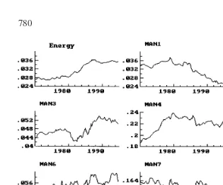
Fig. 1 plots the evolution of employment shares in Italy for 10 two-digit industries (eight manufacturing industries plus energy products and construction).2 Reallocation is clearly evident by the distinct
trends in the shares. Fig. 1 also illustrates how the composition of employment in the industry sector has been altered in the period examined. The changes have been particularly intense for fabricated metal products and construction, but the distinct evolutions in most industries’ shares (basic metal industries, chemical products, food, beverages and tobacco, energy products) indicate that reallocation has changed the composition of employment over the last two decades. A further characteristic is the variability of the industries’ relative shares through time. To this end, it is interesting to note that much of the variations in employment shares reported in Fig. 1 do not occur in and around recessions.
1See Juselius (1993) for an excellent discussion of the economic motivation underlying some recent developments in the macroeconometric analysis of time series.
Figure 1. Employment Shares in industrial sector: Total Employment51.
In order to measure sectoral shifts in labour demand, we use Neumann-Topel’s employment-based dispersion index. A disper-sion index based on employment was used by Lilien (1982).3He
provided empirical evidence from the post-war United States of a positive correlation between aggregate unemployment rate and a sectoral shift proxy measured by weighted standard deviation of employment across sectors. Although Lilien’s sectoral shift hypothe-sis was substantially accepted in the 1980s, Abraham and Katz (1986) stressed the low power of this proxy in capturing sectoral shifts, as the business cycle is not neutral across different markets: a shift in employment in some sectors might be generated by a
cyclical effect instead of representing the consequence of a perma-nent relative change in labour demand. Thus, sectoral shifts and aggregate demand explanations may be observationally equivalent.4
Neumann and Topel consider Abraham and Katz’s critique and define a new proxy, decomposing the variability of employment shares in two components, with the aim of isolating the “perma-nent” changes in labour demand among sectors from changes due to local cycles or other unpredictable events (transitory effects). A “permanent” change in the distribution across sectors, producing mismatch, increases the unemployment rate in the short run. We use a similar index, based on employment distribution in 10 indus-trial sectors, according to Istat classification (eight manufacturing sectors plus the energy and construction sector).
To construct a measure of sectoral shifts we follow three steps: (a) define a direction of a permanent change; (b) compute the actual difference between current and past employment distribu-tion; (c) determine the least squares projection of (b) onto (a).
Employment shares are defined for each sectorSias the ratio
of sectoral employment to the total industry employmentli, i5
1, 2, . . . 10. Consideringl5(l1,l2, . . . ,l10) a vector of employment
shares, Neumann and Topel define the direction of a “permanent” change in industry composition shift as follows:
Dlˆ 5
o
Eq. (1) represents the difference between moving averages of future and past vectors of employment shares. The parameterssi
stand for smoothly declining weights whileJis the time horizon. In our case, we setsi50.9j, withJ 58 quarters. Given Eq. (1),
the difference between the current and the past employment distri-bution is defined as (Eq. (2)):
Dlt5 lt2
o
Jj51
silt2j. (2)
Considering the difference as a linear combination of a permanent effect and a transitory component we can write that
Dlt5 blˆt1 DlTt; b 5(Dlˆ9Dl/Dlˆ9Dlˆ ).
bDlˆ is the least squares projection of the current changes onto
the vector measuring the direction of “permanent” changes, and
DlT
t is the transitory (orthogonal toDlˆ ) component. In the
Neu-mann-Topel terminology, the vector measuring permanent shifts
is given by the following expression,DlP
t 5 bDlˆ .
When “permanent” shifts are zero, over time each sector keeps its share of employment and each component of DlP
t is zero. If
employment shifts, shares will change in the future compared to the past and, therefore, some components inDlP
t will not be zero.
A measure of the importance of the shifts among sectors is pro-vided by the Euclidean length ofDlP
t (3)):
where li is a component of DlPt corresponding to the sector i.
The scalardtis our sectoral shift variable. Its length varies from
0 to
√
2.The choice of s in the smoothing procedure described above seems to be important in describing the behaviour ofdt. Although
changes in the time horizon and in the weights may provide a certain effect on the sectoral shifts measure, we finddtappropriate
to take into account some peculiarities of the sample period.5
2.1. The Dispersion Measuredt
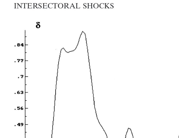
Fig. 2 presents the dispersion measuredt, constructed from
Neu-mann and Topel’s measure of sectoral shifts. Since data are quar-terly, over the period 1973:1–1995:3, the measure is constructed for the period 1975:1–1993:3. The higher its value, the greater is the permanent shift in composition. The importance of sectoral shifts seems to vary considerably over time.dtshows four major
changes in the distribution of employment. A striking and pro-longed “permanent” shift in sectoral composition occurs in the period 1973–1977, while three important, but less remarkable, shifts peak in the periods 1980–1981, 1986–1987 and 1991–1992. The dispersion measure indicates that cross-industry dispersion
Figure 2. Sectoral shift Variable.
of employment growth rates were growing simultaneously with a decline of economic activity (industrial production and GDP) in the first, second and fourth period, whereas the third period (1986–1987) was characterized by marked economic vitality.
The allocative effects due to raw material and oil price shocks can explain the large shifts increases between 1973 and 1977 (evi-dence of the allocative effects of oil price shocks is given in Hamil-ton, 1983; Loungani, 1986; Keane & Prasad, 1996, among others). Moreover, firms were proceeding with a capital-intensive adjust-ment process related to the significant wage increases that occurred in the late 1960s.
exchange rate revaluation effect provides compelling support for the sectoral shifts view also in the last peak, which gives evidence of the rationalization of the productive process, with a reduction of investments and employment.
Some authors (e.g., Davis, 1987b; Hamilton, 1983) stress that reallocation in response to a sectoral disturbance will occur when the economy is in a low state and the opportunity cost is smallest. Rissman (1993), according to this “reallocation timing argument”, emphasizes that it would make unemployment Granger-causing dispersion to the extent that the unemployment rate also reflects cyclical disturbances. Our dispersion measuredtdoes not seem to
give full support to this hypothesis, relating allocative disturbances with an expansionary phase. Below, we use a VAR model to show that an innovation in unemployment variable has no effect on the other variables. That is, unemployment does not Granger-cause the structural shift measure.
3. COINTEGRATION ANALYSIS
3.1. The I(1) Model for Cointegration
We consider a general vector autoregressive model for an -dimen-sional vector processxt. When the data areI(1) a useful reformula-tion of the model is to error correcreformula-tion form:
Dxt5 G1Dxt211 G2Dxt221 Pxt211φDt1εt. (4)
The errors are assumed to be independent Gaussian variables with mean zero and variance o. Dt is a vector of deterministic terms (constants, linear terms, intervention dummies). The lag length in Eq. (4) corresponds to the actual lag length of the VAR models discussed below, and has been determined by some infor-mation criteria. Starting from a VAR with four lags on all stochas-tic variables, simplification tests suggested that three lags sufficed (see Lu¨tkepohl, 1991, for a survey of the criteria).
P5 ab9 has reduced rankranda andbare (n3r) matrices. Johansen shows that the reduced rank of II implies that the sto-chastic part of b9x is stationary and, therefore, with this model we can consider the economic relationsbx 5 jand assume that the agents react to the disequilibrium errorbxt212 jthrough the
The representation theorem of Granger (a way of finding the MA representation from the AR representation, and vice versa, see Johansen, 1995) shows that the solution of Eq. (4) is given by:
xt5 x01C(1)
so
a⊥andb⊥are orthogonal complements ofaandb, respectively. The orthogonal complement ofb,b⊥is defined as the (n3(n2
the deterministic part of the process (e.g., Johansen, 1994). It is seen from Eq. (5) that the cumulative shocksa⊥9ot
i51eidrive
the economic variables to lie in the space spanned by b⊥ (the attractor set). The matrix C(1) describes how the stochastic and deterministic trends determine the long-run components ofx. This matrix is of reduced rank and we will see below that, in our case, it implies that there existn2r54 common trends (a geometrical representation of a simplified version of the space spanned byb⊥
is reported in Appendix A).
A necessary condition for theI(1) model (5) is thata⊥9Gb⊥has full rank (otherwise the processx is integrated of second order). In both models (4) and (5), restrictions are required to identify, respectively, uniquely relations and trends (i.e., Ifb9is a cointegra-tion matrix, so isFb9 with any non-singularr 3 rF).
To identify uniquely the individual long-run relations, it is usual formulate linear restrictionRias full rank matrices (n3ri),Ribi5
0,i51, . . . ,r. Johansen and Juselius (1994) define a matrix (n3
(n2ri)),Hi5Ri⊥and conveniently writeb 5Hiφifor somen3
ridimensional vectorφ. The matrix Hireflects linear (economic)
hypotheses to be tested against the data. This allows to write the rank-condition for identifying the equations. In the cointegration analysis below, we findr 52 stationary relations, which requires the following conditionrij 5r(R9iHj) >1, i?j.
3.2. The Data Set
Data are quarterly, seasonally adjusted over the period 1975:1– 1993:3. The system is in six stochastic variablesx9 5[(w2p),p, (p 2 q), h, U, d].6 The variables are, respectively, consumption
real wage, labour productivity (value added/labour units), price wedge (consumption price minus product price), worked hours, unemployment rate and the sectoral shift variable defined above. The variables refer to the industry sector while the worked hours variable is a proxy, being per capita hours worked in the “large firms” (firms with more than 500 employees). All the variables are in log form, except for the sectoral shift variabledt. Finally, all
the variables are non-stationary (I(1)) time series (the univariate evidence is provided in the JPM website version).7
3.3. The Cointegration Space and the Natural Rate of Unemployment
Using a VAR(3) model and Johansen’s tests and ML estimation method (Johansen, 1988; Johansen & Juselius, 1990), two cointe-gration relations were found.8 The variables characterize most
empirical works based on the bargaining framework. In searching for a restricted cointegrating space, we set down a stylized version of the battle of the mark-ups approach to the natural rate of unemployment.
It is well known that this model makes the wage equation un-identified (Bean, 1994; Manning, 1993). Suppose that wage-setting and pricing equation are estimated in the following form:
6There is a vast literature on seasonal adjustment and the impact of SA on cointegrated time series (e.g., Franses, 1996). In particular, the application of linear moving average filters may yield non-invertible MA processes for the SA time series. Similar results hold for Census X-11 corrected time series (the seasonal adjustment method often applied in practice). See Maravall (1995) for a discussion of the non-invertibility of SA time series). 7The degree of integratedness of the unemployment rate and the sectoral shift variable may be considered a bit puzzling: in fact, both the variables are bounded and seem to be I(1). However, the unemployment rate rises significantly during the last 20 years, changing its average level (see Fig. 2 fordt). Moreover, the order of integration is a statistical
property of the series within the considered sample and not necessarily a property of the generating process.
8The following multivariate tests show the congruency of the initial general system: vectAR(1,5): F(180,108) 5 1.246[0.106]; vectNorm: x2(12) 5 8.657[0.732]; vectHet:
(w2p)5 m01 m1U1 m2X11 m3X2 (6)
(w2p)5φ01φ1X1 (7)
where the vector X1 contains demand side variables and X2is a
vector of variables like union power and other variables that determine wage pressure. As stressed by Manning (see also Westa-way, 1996), even if the cross-equation restrictionsm2X15 2φ1X1
are imposed, so that the invariance of the natural rate of unemploy-ment to demand factors holds, Eq. (6) remains unidentified. This is easily seen from the fact that adding a multiple of the price-setting equation to the wage equation alters only the coefficients of the wage-setting schedule (Eq. (6)):
(w2p)5 s01 s1U1 s2X11 s3X2 (8)
wheres05 Fm02(12 F)φ0;s15 Fm1;s25 Fm22(12 F)φ1;
s35 Fm3; 0, F ,1 (for a critical analysis, see Chiarini & Piselli,
2000).
In this context, the multivariate cointegration approach may play a new role in ensuring that the wage-price structure defined does not suffer from the potential lack of identification of wage-setting relations.
The statistical model was checked to be “identifying” (see Jo-hansen & Juselius, 1994). Subsequently, further restrictions on the parameters space were imposed and tested, obtaining the following LR test, x2(3) 5 2.763[0.4296]. The restrictions placed
on the two vectors are as follows: three restrictions onb1,
compris-ing two zero constraint ((p2q)50 andU50) and a homogeneity constraint ((w2p) 5 p). There are also two restrictions placed on b2, (w 2 p) 5 p and d 5 0. These restricted cointegration
vectors were tested for lying in the cointegration space, jointly with testing for labour productivity and unemployment being weakly exogenous. We found the productivity variable exogenous to the system (x2(6) 55.635[0.4653]).
(t-statistic in parentheses). A simplified geometrical representa-tion of this cointegrarepresenta-tion space is provided in Appendix A.
It is important to emphasize thatUtis weakly exogenous. This
along the attractor set by the common trends, does not react to the disequilibrium error b9xt via the adjustment coefficients. Of
course, this does not mean that Ut does not move together the
others variables (see Johansen, 1992).
In the cointegration space defined by the two stationary rela-tions, unemployment allows a long-run equilibrium between the bargained real wage and the demand of employers (the feasible real wage). It is worth stressing that setting the unemployment restrictions equal to zero in both the cointegrating vectors, pro-vides non-stationary relationships among the variables.
Restricting the demand factors in the price and wage equation to be the same with opposite sign does not provide an acceptable result in terms of LR test. However, our stationary relations iden-tify wage and price-setting schedules without relying on arbitrary (or ad hoc) identifying exclusion restrictions (see Manning, 1993). The first cointegrating vector, Eq. (9), may be interpreted as a price equation. It will depend on unit labour cost, a measure of intrasectoral labour reallocation and a constant (that, for instance, can be related to the degree of product market competition). Labour reallocation tends to determine a lower real wage that, for given productivity, price setters are willing to concede. The second stationary relation (Eq. (10)) may be interpreted as a structural equation for the mark-up of real wages (labour share) that depends negatively on the unemployment rate and prices wedge. In the context of Eqs. (6) and (7), we have:
(w2p)5 s02 s1u1 s2X11 s3X21 s4d (11)
wheres45(12 F)φ2. Clearly, Eq. (11) does not have the same
form as the original wage-setting schedule (Eq. (6)). However, it is important to stress that the stationary relations (9) and (10) cannot be interpreted individually, ignoring the whole system. That is, the short-run dynamics and the adjustment processes (see Chiarini & Piselli, 2000; Lu¨tkepohl, 1991). Below, we return to this problem using impulse responses analysis.
Notice that both the equations constitute testable questions as to whether the hypothetical relation can be assumed to lie in the stationary part of the space spanned by the non-stationary variables. The likelihood ratio tests indicate that stationarity has to be rejected in all the alternative cases.
3.4. An Economic Interpretation
structural shifts. This result seems to question the sectoral shifts hypothesis as a phenomena associated with temporary conse-quences of intersectoral shocks. In fact, it shows that the shifting composition effect of labour demand does not net out on average, influencing the stationary space (wage and unemployment) in the long run (although the service sector, in the period examined, absorbed much of industry’s loss, the reallocation shocks affected the unemployment rate). As we shall see below, taking the short-term dynamics into account and carrying out the impulse response analysis provides a similar conclusion. Thus, more than frictional (or transitional) unemployment related to individuals changing jobs across sectors, we obtain a persistent imbalance between supply of and demand for labour across sectors. Increased mis-match reflects the failure of relative wages to adjust or inadequate mobility.
This (long-run) mismatch phenomenon is perhaps more worthy of study than the conventional composition hypothesis with short-run turbulence, and it arises essentially from the supply side. The literature on Italian labour market mobility seems to provide support for these results: low workforce adaptability; low willing-ness to change employment status; high retraining costs; low geo-graphical mobility; high employment protection regulations on hiring and firing; high inefficiency of public placement offices (see among others, Attanasio & Padoa Schioppa, 1991; De Luca & Bruni, 1993; Galli et al., 1996; OECD, 1995).
These institutional and labour market features, along with infor-mational mismatches between workers and firms and other barri-ers to short-run labour mobility, increase the difficulty of re-estab-lishing an efficient pattern of matches between firms and workers across sectors.
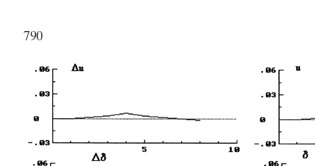
Figure 3. Impulse response on sectoral shift.
during collective bargaining (see, for instance, Erikson & Ichino, 1994). At least until the mid-1980s, intersectoral (and regional) wage differentials narrowed, and wage dispersion in manufactur-ing picked up in the second half of the decade, but in the first years of the 1990s, its value did not reach that obtained at the beginning of the 1970s. Thus, although wage levelling has been opposed by employers by using wage drift, the sectoral shifts could not produce downward wage pressures in some sectors and, as a reaction, upward wage pressures in others.
4. IMPULSE RESPONSE FUNCTIONS
Having determined the cointegration space, we reformulate and estimate (by FIML) the model using a general to specific modelling approach and imposing specific restrictions on each equation (the model is reported in the JPM website version).
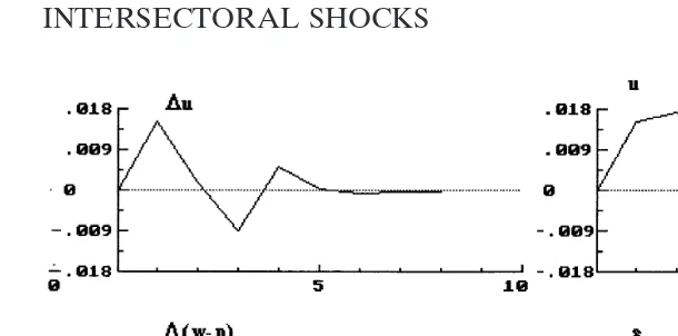
Figure 4. Impulse response on real wage.
Consistent with a key prediction of the sectoral shifts literature, we find that an unfavourable allocative disturbance increases aggre-gate unemployment in the short run, but it does reduce employment persistently, shifting industry employment shares in the long run.9
These findings imply a low rate of job reallocation and indicate a difficult reshuffling of employment opportunities across sectors, with persistent sectoral-level employment changes. This may indi-cate that job substitution is typically associated with long-term joblessness.
It is interesting to note that a transitory wage shock is estimated to account for most of the long-run behaviour of unemployment, giving rise to a permanent shift in the composition of labour demand. On the other hand, there is no significant short-run or permanent effect on real wage due to an innovation in the shift variable, although the latter leads to a long-term increase in unem-ployment. Real wage rigidity and a more rapid structural shift tends to introduce inertia into the firms’ employment decision, raising the flows of people into unemployment and increasing the pool of those who are unemployed between jobs.
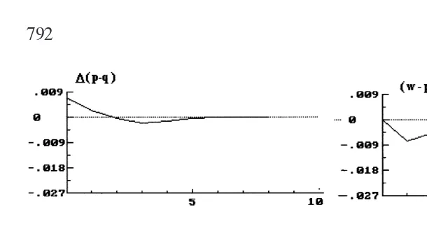
Figure 5. Impulse response on relative prices.
5. POLICY IMPLICATIONS
From the policy perspective there are two important questions that arise from the empirical evidence produced in this paper. First, our results suggest that fluctuations due to intersectoral job allocations are important for the NAIRU. However, stylized versions of the textbook approach to the NAIRU, whereby unem-ployment must move to equilibrate the demands of employers and the bargaining real wage (as in the battle of the mark-ups
framework) are strongly deceptive. NAIRU estimates, obtaining by using the conventional reduced form (or Phillips curve) models, are incorrect since the natural rate of unemployment cannot con-sidered as a fixed point, calling for the ceteris paribus assumption for all the data involved. This implies that the NAIRU estimates are unable to provide valuable information on the labour market status. In fact, these models do not perform any analysis of the joint distribution of the set of random variables involved (that is, an adequate description of the data generation process). As a result, point estimates vary greatly (see Staiger, Stock, & Watson, 1996) and the NAIRU indicator cannot be considered a useful concept in policy formulation. Thus, the empirical evidence based on these solutions are seriously misspecified and the policy impli-cations erroneous.
fact that the reduced form (the statistical model that comprises the probability model and the sampling model and that forms the basis of the parametric inference) is not estimated explicitly (see, Chiarini & Piselli, 2000; Spanos, 1989, 1990). We have shown in the paper that, considering a VAR representation as form of the joint data density function, the use of multivariate cointegration approach provides a new role for the identification problem, lead-ing to a greatly complicated and enriched NAIRU model. The simplified version of the geometrical representation of the NAIRU reported in Figs. A1 and A2, shows that the NAIRU is not a fixed point but a solution in a stationary space. The MA representation (Eq. (5)) of the VAR model emphasizes how a random shock to an equation of the model produces random short-run effects (via
C(L)εt) and long-run effects (viaC(1)εt), engendering a new posi-tion in the space spanned by the attractor set. A shock to one variable implies a shock to all the variables in the long run: in this context, the ceteris paribus assumption is not allowed, the only way of analyzing the economic relationships remains the impulse response functions. This framework brings out a key pol-icy point: claims such as,
in the long-run, unemployment is determined entirely by long-run supply factors and equals the NAIRU; in the short-run, unemployment is deter-mined by the interaction of aggregate demand and short-run aggregate supply (Layard et al., 1991)
are misleading.
As an example, we show in Fig. 5 a result that emerge from our study: the striking effect of the price wedge changes on dispersion measure and, therefore, on unemployment. An increase of a one-time (one standard deviation) impulse in the price wedge is seen to have a lasting effect on sectoral mismatch and unemployment. Although unemployment changes taper off to zero quite rapidly, the unemployment level does not die out asymptotically. Real wage and, therefore, unemployment responses will result in lower equilibrium values.
The second issue raises the question of which policy should be attempted. The results suggest that the sectoral distribution of employment changes is important for both the short and the long-run unemployment performance. The picture that one should have in mind is that the continuous process of disturbances and sectoral job reallocation produce unemployment persistence. While it can be argued that macroeconomics policies have an important role to play in attenuating negative disturbances to the economy (we emphasize again that an uncritical bargaining framework is prob-lematic for this purpose), it appears reasonable to state that struc-tural policies have a central role in acting on those factors that produce and enhance mismatch problems in the economy.
Because of industry-specific skills and a labour market situation characterized by institutional rigidities, with a plethora of regula-tions and a climate of resistance to change (see the literature quoted in Section 3), the process of labour reallocation between different sectors of industry involves temporary mismatches but also provides an important source of the persistence of unemployment.
Moreover, the impulse response functions in Fig. 4 show that not only should considerable efforts be made in employment and redundancy legislation areas and working-time arrangements, but also changes in wage-setting procedures are required to accommo-date structural unemployment. Mismatching of jobs and workers may raise both vacancies and unemployment. However, if wages rise quickly in expanding demand sectors there is no reason to believe that the slow (if any) adjustment to intersectoral shift of labour demand will lead to firms with more capital-intensive.
The impulse responses suggest that a reallocation distribution variable plays a significant role in short-run adjustment and long-run consequences of unemployment to wage and price shocks: wage policy agreements between both sides of industry and gov-ernment may be useful to moderate wage increases in the context of a growth policy based on investment, employment and labour market programmes.
6. CONCLUDING REMARKS
The result that is more interesting and more worthy of comment is that permanent shifts in the composition of employment lead to permanent (in contrast with transitory) increases in unemploy-ment. Permanent sectoral shifts are significant determinants of unemployment. Given the real wage process, our results make extreme Lilien’s view that sectoral shifts are a prime factor gener-ating long lasting (rather than cyclical fluctuations) effects in job-lessness. This result seems to contradict other analysis carried out for Italian unemployment that emphasizes that the potential explanatory power of mismatch and structural imbalances by in-dustry, relative to unemployment, is very modest.10
Finally, from the statistical point of view, one of the main effects of includingdtin the data set is to cancel the need to utilize dummy
variables in the model (see the model discussed in Chiarini & Piselli, 1997). This is not surprising sincedtaccounts for the
struc-tural change effects in the period. All this is obtained with better stochastic properties.
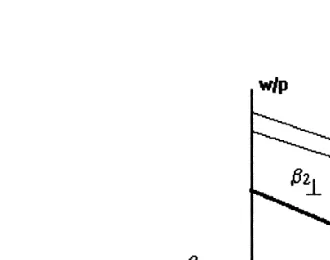
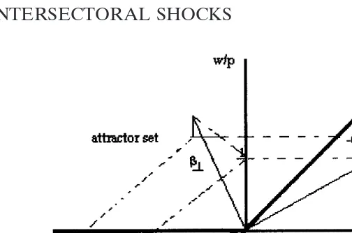
APPENDIX A:
The attractor set b⊥ (the space within which the cointegrated variables move) is a hyperplane with dimension n 2 r 5 4 (six
Figure A1. Stationary Planes inR3.
variables and two cointegration vectors). For the purposes of this exposition, a geometrical representation may be provided consid-ering only three variables, say, (w2p),dandU. In thisR3space,
we have the following stationary relations: (w 2 p) 5 20.015d
and (w 2p) 5 20.06U, that is:b15(1, 0.015, 0) and b25(1, 0,
0.06). It is important to stress that the variables labour productiv-ity, price wedge and worked hours are considered only for exposi-tional purposes: the example that is proposed for an attractor for three variables [(w2p),d,U] is represented in Fig. A1. To obtain the attractor spaceb⊥we have to solve the linear system:
1
1 0.015 0 1 0 0.0621
x1
x2
x3
2
50.
This system (three variables and two equations) has∞1solutions.
Consequently, one can achieve only a parametric solution. Fig. A2 shows that in our simplified system, the attractor space is a straight line: the equations describe orthogonal planes, respec-tively, to b1 and b2 and their intersection is a line. The points
along this line are vertex of all vectors with coordinates (l,266.7l,
Figure A2. Attractor Set inR3.
REFERENCES
Abraham K., & Katz L. (1986) Cyclical unemployment: sectoral shifts or aggregate distur-bances?Journal of Political Economy94:507–522.
Attanasio O.P., & Padoa Schioppa F. (1991) Regional inequalities, migration and mismatch in Italy. InMismatch and Labour Mobility(F. Padoa Schioppa, Ed.) Cambridge, UK: Cambridge University Press, (pp. 237–320).
Bean C. (1994) European unemployment: a survey.Journal of Economic Literature32:573– 619.
Blanchard O.J., & Diamond P.A. (1989) The Beveridge curve.Brookings Papers on Economic Activity1:1–60.
Brainard S.L., & Cutler D.M. (1993) Sectoral shifts and cyclical unemployment reconsid-ered.Quarterly Journal of Economics108:219–243.
Campbell J.R., & Kuttner K.N. (1996) Macroeconomic effects of employment reallocation.
Carnegie-Rochester Conference Series on Public Policy44:87–116.
Charette M.F., & Kaufmann B. (1987) Short-run variation in the natural rate of unemploy-ment.Journal of Macroeconomics.9:417–427.
Chiarini B., & Piselli P. (1997) Wage setting, wage curve and Phillips curve: the Italian evidence.Scottish Journal of Political Economy44:545–565.
Chiarini B., & Piselli P. (2000) Identification and dimension of the NAIRU. Economic Modelling, forthcoming.
Cross R., & Darby J. (1996) Hysteresis and ranges or intervals for equilibrium unemploy-ment.EUI, Robert Schuman Centre Working Papers, 1–37.
Davis S.J. (1987a) Fluctuations in the pace of labor reallocation.Carnegie-Rochester Confer-ence Series on Public Policy27:335–402.
Davis S.J. (1987b) Allocative disturbances and specific capital in real business cycle theories.
American Economic Review, Papers and Proceedings77:326–332.
Davis S.J., & Haltiwanger J. (1992) Gross job creation, cross job destruction, and employ-ment reallocation.Quarterly Journal of Economics107:819–863.
Elmeskov J. (1993) High and persistent unemployment: assessment of the problem and its causes.OECD Working Paper132:1–119.
Erikson C.L., & Ichino A. (1996) Wage differentials in Italy: market forces, institutions, and inflation.NBER Working Paper4922:1–44.
Franses P.H. (1996) Periodicity and stochastic trends in economic time series.Oxford: Oxford Univ. Press.
Galli G., Faini R., Rossi F., & Gennari P. (1996) An empirical puzzle: falling migrations and growing unemployment differentials among Italian regions.EUI, Robert Schuman Centre Working Papers1–11.
Hamilton J.D. (1983) Oil and macroeconomy since World War II.Journal of Political Economy91:1232–1266.
Johansen S. (1988) Statistical analysis of cointegration vectors.Journal of Economic Dy-namics and Control12:231–254.
Johansen S. (1992) Testing weak exogeneity and the order of cointegration in UK money demand data.Journal of Policy Modeling14:313–334.
Johansen S. (1994) The role of the constant and linear terms in cointegration analysis of nonstationary variables.Econometric Review13:205–229.
Johansen S. (1995)Likelihood-based inference in cointegrated vector autoregressive models.
Oxford: Oxford Univ. Press.
Johansen S., & Juselius K. (1990) Maximum likelihood estimation and inference on cointe-gration. With applications to the demand for money.Oxford Bulletin of Economics and Statistics52:169–210.
Johansen S., & Juselius K. (1994) Identification of the long-run and the short-run structure. An application to the ISLM model.Journal of Econometrics63:7–36.
Juselius K. (1993) VAR modelling and Haavelmo’s probability approach to macroeconomic modelling.Empirical Economics18:595–622.
Keane M.P., & Prasad E.S. (1996) The employment and wage effects of oil price changes: a sectoral analysis.Review of Economics and Statistics78:389–399.
Layard R., Nickell S. & Jackman A. (1991)Unemployment. Oxford: Oxford University Press.
Lilien D. (1982) Sectoral shifts and cyclical unemployment.Journal of Political Economy
90:777–793.
Lilien D., & Hall R.E. (1986) cyclical fluctuations in the labor market. InHandbook of labor economics. (O. Ashenfelter, & R. Layard, Eds.) Amsterdam: Elsevier (pp. 1001–1035).
Loungani P. (1986) Oil price shocks and the dispersion hypothesis.Review of Economics and Statistics68:536–539.
Loungani P, Rush M., & Tave W. (1990) Stock market dispersion and unemployment.
Journal of Monetary Economics25:367–388.
Lu¨tkepohl H. (1991)Introduction to multiple time series analysis. Berlin: Springer-Verlag. Lu¨tkepohl H., & Reimers H.-E. (1992) Impulse response analysis of cointegrated systems.
Journal of Economic Dynamics and Control16:53–78.
Manning A. (1993) Wage bargaining and the Phillips curve: the identification and specifica-tion of aggregate wage equaspecifica-tions.Economic Journal103:98–118.
Maravall A. (1995) Unobserved components in economic time series. InHandbook of Applied Econometics. (M.H. Pesaran, & M. Wickens, Eds.). Oxford: Blackwell Handbooks in Economics, (pp. 12–72).
Neumann G.R., & Topel R.H. (1991) Employment risk, diversification, and unemployment.
OECD (1995).The OECD jobs study: taxation, employment and unemployment. Paris: OECD.
OECD (1997)Implementing the OECD jobs strategy. Members countries; experience.Paris: OECD.
Padoa Schioppa F. (Ed.). (1991)Mismatch and labour mobility. Cambridge: Cambridge Univ. Press.
Palley T.I. (1992) Sectoral shifts and cyclical unemployment. A reconsideration.Economic Inquiry30:117–133.
Phelps E.S., & Zoega G. (1998) Natural-rate theory and OECD unemployment.Economic Journal108:782–801.
Pissarides C.A. (1990)Equilibrium unemployment theory. Oxford: Blackwell.
Rissman E.R. (1993) Wage growth and sectoral shifts. Phillips curve redux.Journal of Monetary Economics31:395–416.
Spanos, A. (1989) On re-reading Haavelmo: a retrospective view of econometric modeling.
Econometric Theory5:405–429.
Spanos, A. (1990) The simultaneous equations model revisited.Journal of Econometrics
44:87–105.
Staiger D., Stock J.H., & Watson M.W. (1996) How precise are estimates of the natural rate of unemployment?NBER Working Paper5477:1–58.