arXiv:0904.4175v2 [math.PR] 12 Jul 2010
ROMAIN ABRAHAM AND JEAN-FRANC¸ OIS DELMAS
Abstract. We present a construction of a L´evy continuum random tree (CRT) associated with a super-critical continuous state branching process using the so-called exploration pro-cess and a Girsanov theorem. We also extend the pruning procedure to this super-critical case. Let ψ be a critical branching mechanism. We set ψθ(·) = ψ(·+θ)−ψ(θ). Let Θ = (θ∞,+∞) or Θ = [θ∞,+∞) be the set of values ofθ for whichψθ is a conservative branching mechanism. The pruning procedure allows to construct a decreasing L´evy-CRT-valued Markov process (Tθ, θ∈Θ), such that Tθ has branching mechanism ψθ. It is
sub-critical ifθ >0 and super-critical if θ <0. We then consider the explosion time A of the CRT: the smallest (negative) timeθ for which the continuous state branching process (CB) associated withTθ has finite total mass (i.e. the length of the excursion of the exploration
process that codes the CRT is finite). We describe the law ofAas well as the distribution of the CRT just after this explosion time. The CRT just after explosion can be seen as a CRT conditioned not to be extinct which is pruned with an independent intensity related toA. We also study the evolution of the CRT-valued process after the explosion time. This extends results from Aldous and Pitman on Galton-Watson trees. For the particular case of the quadratic branching mechanism, we show that after explosion the total mass of the CB behaves like the inverse of a stable subordinator with index 1/2. This result is related to the size of the tagged fragment for the fragmentation of Aldous’ CRT.
1. Introduction
Continuous state branching processes (CB in short) are non-negative real valued Markov processes first introduced by Jirina [20] that satisfy a branching property: the process (Zt, t≥
0) is a CB if its law when starting fromx+x′is equal to the law of the sum of two independent copies ofZ starting respectively fromxand x′. The law of such a process is characterized by the so-called branching mechanism ψvia its Laplace functionals. The branching mechanism
ψ of a CB is given by
ψ(λ) = ˜αλ+βλ2+
Z
(0,+∞)
π(dℓ)he−λℓ−1 +λℓ1{ℓ≤1}i,
where ˜α ∈R,β ≥0 and π is a Radon measure on (0,+∞) such thatR
(0,+∞)(1∧ℓ2)π(dℓ)<
+∞. The CB is said to be respectively sub-critical, critical, super-critical when ψ′(0) >0,
ψ′(0) = 0 or ψ′(0)<0. We will write (sub)critical for critical or sub-critical. Notice that ψ
is smooth and strictly convex if β >0 orπ 6= 0.
It is shown in [21] that all these CBs can be obtained as the limit of renormalized sequences of Galton-Watson processes. A genealogical tree is naturally associated with a Galton-Watson process and the question of existence of such a genealogical structure for CB arises naturally.
Date: July 13, 2010.
2000Mathematics Subject Classification. 60J25, 60G55, 60J80.
Key words and phrases. Continuum random tree, explosion time, pruning, tree-valued Markov process, continuous state branching process, exploration process.
This question has given birth to the theory of continuum random trees (CRT), first introduced in the pioneer work of Aldous [8, 7, 9]. A continuum random tree (called L´evy CRT) that codes the genealogy of a general (sub)critical branching process has been constructed in [23, 24] and studied further in [17]. The main tool of this approach is the so-called exploration process (ρs, s∈R+), whereρsis a measure onR+, which codes for the CRT. For (sub)critical
quadratic branching mechanism (π = 0), the measure ρs is just the Lebesgue measure over
an interval [0, Hs], and the so-called height process (Hs, s∈R+) is a Brownian motion with
drift reflected at 0. In [16], a CRT is built for super-critical quadratic branching mechanism using the Girsanov theorem for Brownian motion.
We propose here a construction for general super-critical L´evy tree, using the exploration process, based on ideas from [16]. We first build the super-critical tree up to a given level
a. This tree can be coded by an exploration process and its law is absolutely continuous with respect to the law of a (sub)critical L´evy tree, whose leaves above level aare removed. Moreover, this family of processes (indexed by parametera) satisfies a compatibility property and hence there exists a projective limit which can be seen as the law of the CRT associated with the super-critical CB. This construction enables us to use most of the results known for (sub)critical CRT. Notice that another construction of a L´evy CRT that does not make use of the exploration process has been proposed in [19] as the limit, for the Gromov-Hausdorff metric, of a sequence of discrete trees. This construction also holds in the super-critical case but is not easy to use to derive properties for super-critical CRT.
In a second time, we want to construct a “decreasing” tree-valued Markov process. To begin with, if ψ is (sub)critical, for θ > 0 we can construct, via the pruning procedure of [5], from a L´evy CRT T associated with ψ, a sub-tree Tθ associated with the branching
mechanismψθ defined by
∀λ≥0, ψθ(λ) =ψ(λ+θ)−ψ(θ).
By [1, 25], we can even construct a “decreasing” family of L´evy CRTs (Tθ, θ ≥0) such that
Tθ is associated with ψθ for everyθ≥0.
In this paper, we consider a critical branching mechanism ψ and denote by Θ the set of real numbersθ(including negative ones) for whichψθis a well-defined conservative branching
mechanism (see Section 5.3 for some examples). Notice that Θ = [θ∞,+∞) or (θ∞,+∞) for someθ∞∈[−∞,0]. We then extend the pruning procedure of [5] to super-critical branching mechanisms in order to define a L´evy CRT-valued process (Tθ, θ∈Θ) such that
• For every θ∈Θ, the L´evy CRT Tθ is associated with the branching mechanism ψθ.
• All the trees Tθ,θ∈Θ have a common root.
• The tree-valued process (Tθ, θ∈Θ) is decreasing in the sense that for θ < θ′,Tθ′ is a
sub-tree of Tθ.
Letρθbe the exploration process that codes forT
θ. We denote byNNNψthe excursion measure
of the process (ρθ, θ∈Θ), that is underNNNψ, eachρθ is the excursion of an exploration process
associated withψθ. Letσθ denote the length of this excursion. The quantity σθ corresponds
also to the total mass of the CB associared with the treeTθ. We say that the tree Tθ is finite
(underNNNψ) ifσθ is finite (or equivalently if the total mass of the associated CB is finite). By
construction, we have that the treesTθ forθ≥0 are associated with (sub)critical branching
mechanisms and hence are a.e. finite. On the other hand, the trees Tθ for negative θ are
associated with super-critical branching mechanisms. We define the explosion time
Forθ∈Θ, we define ¯θas the unique non-negative real number such that
(1) ψ(¯θ) =ψ(θ)
(notice that ¯θ=θ if θ ≥0). If θ∞6∈Θ, we set ¯θ∞= limθ↓θ∞θ¯. We give the distribution of
A underNNNψ (Theorem 6.5). In particular we have, for allθ∈[θ∞,+∞), N
NNψ[A > θ] = ¯θ−θ.
We also give the distribution of the trees after the explosion time (Tθ, θ ≥A) (Theorem 6.7
and Corollary 8.2). Of particular interest is the distribution of the tree at its explosion time, TA.
The pruning procedure can been viewed, from a discrete point of view, as a percolation on a Galton-Watson tree. This idea has been used in [11] (percolation on branches) and in [4] (percolation on nodes) to construct tree-valued Markov processes from a Galton-Watson tree. The CRT-valued Markov process constructed here can be viewed as the contiuous analogue of the discrete models of [11] and [4] (or maybe a mixture of both constructions). However, no link is actually pointed out between the discrete and the continuous frameworks.
In [11] and [4], another representation of the process up to the explosion time is also given in terms of the pruning of an infinite tree (a (sub)critical Galton-Watson tree conditioned on non-extinction). In the same spirit, we also construct another tree-valued Markov process (T∗
θ, θ ≥0) associated with a critical branching mechanism ψ. In the case of a.s. extinction
(that is when
Z +∞ dv
ψ(v) < +∞), T0∗ is distributed as T0 conditioned to survival. The tree T∗
0 is constructed via a spinal decomposition along an infinite spine. Then, we define
the continuum-tree-valued Markov process (T∗
θ, θ ≥ 0) again by a pruning procedure. Let
θ ∈ (θ∞,0). We prove that under the excursion measure NNNψ, given A = θ, the process
(Tθ+u, u≥0) is distributed as the process (Tθ+u¯∗ , u≥0) (Theorem 8.1).
When the branching mechanism is quadratic, ψ(λ) = λ2/2, some explicit computations can be carried out. Let σθ∗ be the total mass of T∗
θ and τ = (τθ, θ ≥0) be the first passage
process of a standard Brownian motion, that is a stable subordinator with index 1/2. We get (Proposition 9.1) that (σ∗θ, θ ≥0) is distributed as (1/τθ, θ ≥0) and that (σA+θ, θ ≥0)
is distributed as (1/(V +τθ), θ ≥0) for some random variable V independent of τ. Let us
recall that the pruning procedure of the tree can be used to construct some fragmentation processes (see [6, 1, 25]) and the process (σθ, θ≥0), conditionally onσ0= 1, represents then
the evolution of a tagged fragment. We hence recover a well known result of Aldous-Pitman [10]: conditionally onσ0 = 1, (σθ, θ ≥0) is distributed as (1/(1 +τθ), θ≥0) (see Corollary
9.2).
The paper is organized as follows. In Section 2, we introduce an exponential martingale of a CB and give a Girsanov formula for CBs. We recall in Section 3 the construction of a (sub)critical L´evy CRT via the exploration process and some useful properties of this exploration process. Then, we construct in Section 4 the super-critical L´evy CRT via a Girsanov theorem involving the same martingale as in Section 2. We recall in Section 5 the pruning procedure for critical or sub-critical CRTs and extend this procedure to super-critical CRTs. We construct in Section 6 the tree-valued process (Tθ, θ ∈ Θ), or more precisely
the family of exploration processes (ρθ, θ ∈ Θ) which codes for it. We also give the law of the explosion time A and the law of the tree at this time. In Section 7, we construct an infinite tree and the corresponding pruned sub-trees (T∗
θ, θ ≥ 0), which are given by a
(TA+u, u≥0) is distributed as the process (TU+u∗ , u≥0) whereU is a positive random time
independent of (T∗
θ , θ≥0). We finally make the explicit computations for the quadratic case
in Section 9.
Notice that all the results in the following Sections are stated using exploration processes which code for the CRT, instead of the CRT directly. An informal description of the links between the CRT and the exploration process is given at the end of Section 3.6.
2. Girsanov formula for continuous branching process
2.1. Continuous branching process. Letψbe a branching mechanism of a CB: forλ≥0, (2) ψ(λ) = ˜αλ+βλ2+
Z
(0,+∞)
π(dℓ)he−λℓ−1 +λℓ1{ℓ≤1}i,
where ˜α∈R,β≥0 and π is a Radon measure on (0,+∞) such that R
(0,+∞)(1∧ℓ2)π(dℓ)<
+∞. We shall say that ψ has parameter (˜α, β, π).
We shall assume thatβ6= 0 orπ 6= 0. We haveψ(0) = 0 andψ′(0+) = ˜α−R
(1,+∞)ℓπ(dℓ)∈
[−∞,+∞). In particular, we have ψ′(0+) = −∞ if and only if R
(1,+∞)ℓ π(dℓ) = +∞. We
say that ψis conservative if for all ε >0
(3)
Z ε
0
1
|ψ(u)| du= +∞. Notice that (3) is fulfilled ifψ′(0+)>−∞that is ifR
(1,+∞)ℓ π(dℓ)<+∞. Ifψis conservative,
the CB associated withψ does not explode in finite time a.s.
Let Pψx be the law of a CBZ= (Za, a≥0) started atx≥0 and with branching mechanism
ψ, and let Eψx be the corresponding expectation. The processZ is a Feller process and thus
has a c`ad-l`ag version. Let F = (Fa, a ≥ 0) be the filtration generated by Z completed the
usual way. For every λ >0, for everya≥0, we have
(4) Eψxhe−λZai= e−xu(a,λ),
where functionu is the unique non-negative solution of
(5) u(a, λ) +
Z a
0
ψ u(s, λ)
ds=λ, λ≥0, a≥0.
This equation is equivalent to
(6)
Z λ
u(a,λ)
dr
ψ(r) =a λ≥0, a≥0.
If (3) holds, then the process is conservative: a.s. for alla≥0,Za<+∞.
Letq0be the largest root ofψ(q) = 0. Sinceψ(0) = 0, we haveq0 ≥0. Ifψis (sub)critical,
since ψ is strictly convex, we get that q0 = 0. If ψ is super-critical, if we denote by q∗ >0
the only real number such that ψ′(q∗) = 0, we have q0 > q∗ > 0. See Lemma 2.4 for the
interpretation of q0.
Iff is a function defined on [γ,+∞), then for θ≥γ, we set for λ≥γ−θ:
fθ(λ) =f(θ+λ)−f(θ).
Ifν is a measure on (0,+∞), then for q∈R, we set
Remark 2.1. If π(q)((1,+∞)) < +∞ for some q < 0, then ψ given by (2) is well defined on [q,+∞) and, for θ∈ [q,+∞), ψθ is a branching mechanism with parameter (˜α+ 2βθ+
R
(0,1]π(dℓ) ℓ(1−e−θℓ), β, π(θ)). Notice that for all θ > q, ψθ is conservative. And, if the
additional assumption
Z
(1,+∞)
ℓπ(q)(dℓ) =
Z
(1,+∞)
ℓe|q|ℓπ(dℓ)<+∞
holds, then |(ψq)′(0+)|<+∞ and ψq is conservative.
2.2. Girsanov formula. Let Z = (Za, a≥ 0) be a conservative CB with branching
mech-anism ψ given by (2) with β 6= 0 or π 6= 0, and let (Fa, a ≥ 0) be its natural filtration.
Let q ∈ R such that q ≥ 0 or q < 0 and R
(1,+∞)ℓe|q|ℓπ(dℓ) < +∞. Then, thanks to
Re-mark 2.1,ψ(q) andψq are well defined and ψq is conservative. Then we consider the process
Mψ,q = (Mψ,q
a , a≥0) defined by
(8) Maψ,q= eqx−qZa−ψ(q)R0aZsds.
Theorem 2.2. Let q∈Rsuch that q≥0 or q <0 andR
(1,+∞)ℓe|q|ℓπ(dℓ)<+∞.
(i) The process Mψ,q is a F-martingale under Pxψ.
(ii) Let a, x≥0. OnFa, the probability measure Pψxq is absolutely continuous with respect
to Pψx and
dPψq
x |Fa
dPψx|Fa
=Maψ,q.
Before going into the proof of this theorem, we recall Proposition 2.1 from [2]. For µ a positive measure onR, we set
(9) H(µ) = sup{r ∈R;µ([r,+∞))>0},
the maximal element of its support. Fora <0, we setZa= 0.
Proposition 2.3. Let µ be a finite positive measure on R with support bounded from above
(i.e. H(µ) is finite). Then we have for all s∈R, x≥0,
(10) Eψxhe−RRZr−sµ(dr)
i
= e−xw(s),
where the function w is a measurable locally bounded non-negative solution of the equation
(11) w(s) +
Z +∞
s
ψ(w(r))dr=
Z
[s,+∞)
µ(dr), s≤H(µ) and w(s) = 0, s > H(µ).
If ψ′(0+) > −∞ or if µ({H(µ)}) > 0, then (11) has a unique measurable locally bounded non-negative solution.
Proof of Theorem 2.2. First case. We considerq >0 such thatψ(q) ≥0.
We have 0≤Maψ,q ≤eqx, thus Mψ,q is bounded. It is clear thatMψ,q is F-adapted.
To check thatMψ,q is a martingale, thanks to the Markov property, it is enough to check
that Eψx[Maψ,q] = Eψx[M0ψ,q] = 1 for all a≥0 and all x≥0. Consider the measure νq(dr) =
qδa(dr) +ψ(q)1[0,a](r)dr, where δa is the Dirac mass at pointa. Notice thatH(νq) =a and
that νq {H(νq)} = q > 0. Hence, thanks to Proposition 2.3, there exists a unique
(11) withµ=νq, we deduce thatw=q1[0,a]and that Ex[Maψ,q] = 1. Thus, we get thatMψ,q deduce that u is non-negative and solves
(12) u(s) + Proposition 2.3, we deduce that u is the unique non-negative solution of (12) and that e−xu(0) = Eψq
x [e−
R
RZrν(dr)]. In particular, we have that for all non-negative measure ν on
Rwith support in [0, a],
As e−RRZrν(dr) isFa-measurable, we deduce from the monotone class theorem that for any non-negativeFa-measurable random variableW,
(13) EψxhW eqx−qZa−ψ(q)R0aZrdri= Eψ
x[W Maψ,q] = E ψq
x [W].
This proves the second part of the theorem.
If q > q∗, formula (13) holds with ψ replaced by ψq∗ and q replaced by q −q∗, which also
yields equation (15).
Using (14), (15) and that ψq∗(−q∗) +ψ(q) =ψq∗(q−q∗), we get that
ExψhW eqx−qZa−ψ(q)R0aZrdri= Eψq∗
x
h
W e−(q∗−q)x+(q∗−q)Za−(ψq∗(−q∗)+ψ(q))
Ra
0 Zrdri (16)
= Eψq∗
x
h
W e−(q∗−q)x+(q∗−q)Za−ψq∗(q−q∗)
Ra
0 Zrdr
i
= Eψq
x [W].
Since this holds for any non-negative Fa-measurable random variableW, this proves (i) and
(ii) of the theorem.
Third case. We consider q <0 and assume that R
(1,+∞)ℓe|q|ℓ π(dℓ)<+∞. In particular,
ψq is a conservative branching mechanism, thanks to Remark 2.1.
LetW be any non-negativeFa-measurable random variable . Using (13) ifψq(−q)≥0 or
(16) ifψq(−q)<0, with ψreplaced by ψq andq by−q, we deduce that
Eψq
x [We−qx+qZa−ψq(−q)
Ra
0 Zrdr] = Eψ
x[W].
This implies that
Eψq
x [W] = Eψx[W eqx−qZa+ψq(−q)
Ra
0 Zrdr] = Eψ
x[W eqx−qZa−ψ(q)
Ra
0 Zrdr].
Since this holds for any non-negative Fa-measurable random variableW, this proves (i) and
(ii) of the theorem.
Finally, we recall some well known facts on CB. Recall thatq0is the largest root ofψ(q) = 0,
q0 = 0 if ψ is (sub)critical and thatq0>0 if ψ is super-critical. We set
(17) σ=
Z +∞
0
Zada.
Forλ≥0, we set
(18) ψ−1(λ) = sup{r ≥0; ψ(r) =λ}
and we call σ the total mass of the CB.
Lemma 2.4. Assume that ψ is given by (2) with β6= 0 or π6= 0 and is conservative. (i) Then Pψx-a.s. Z∞= lima→+∞Za exists, Z∞∈ {0,+∞},
(19) Pψx(Z∞= 0) = e−xq0, {Z∞= 0}={σ <+∞}and we have: for λ >0,
(20) Eψxhe−λσi= e−xψ−1(λ).
(ii) Let q >0 such that ψ(q)≥0. Then, the probability measure Pψq
x is absolutely
contin-uous with respect to Pψx with
dPψq
x
dPψx
=M∞ψ,q,
where
(iii) If ψ is super-critical then, conditionally on {Z∞ = 0}, Z is distributed as Pψq0: for any non-negative random variable measurable w.r.t. σ(Za, a≥0), we have
Eψx[W|Z∞= 0] = Eψq0
x [W].
Proof. For λ > 0, we set Na = e−λZa+xu(a,λ), where u is the unique non-negative solution
of (6). Thanks to (4) and the Markov property, (Na, a≥0) is a bounded martingale under
Pψx. Hence, as a goes to infinity, it converges a.s. and in L1 to a limit, say N∞. From
(6), we get that lima→+∞u(a, λ) = q0. This implies that Z∞ = lima→+∞Za exists a.s. in
[0,+∞]. Since Eψx[N∞] = 1, we get Eψx[e−λZ∞] = e−q0x for all λ > 0. This implies that
Pψx-a.s. Z∞∈ {0,+∞}and (19).
Clearly, we have {Z∞ = +∞} ⊂ {σ = +∞}. For q > 0 such that ψ(q) ≥0, we get that (Maψ,q, a ≥0) is a bounded martingale under Pψx. Hence, as agoes to infinity, it converges
a.s. and in L1 to a limit, say Mψ,q
∞ . We deduce that
(22) Eψxhe−ψ(q)σ1{Z∞=0}i= e−qx.
Letting q decrease to q0, we get that Pψx(σ <+∞, Z∞= 0) = e−q0x = Pψx(Z∞ = 0). This
implies that Pψx a.s. {σ = +∞} ⊂ {Z∞ = +∞}. We thus deduce that Pψx a.s. {Z∞ =
+∞}={σ = +∞}. Notice also that (21) holds.
Notice that (22) readily implies (20). This proves Property (i) of the lemma and (21). Property (ii) is then a consequence of Theorem 2.2, Property (ii) and the convergence in
L1 of the martingale (Mψ,q
a , a≥0) towards M∞ψ,q.
Property (iii) is a consequence of (ii) withq =q0 and (19).
3. L´evy continuum random tree
We recall here the construction of the L´evy continuum random tree (CRT) introduced in [24, 23] and developed later in [17] for critical or sub-critical branching mechanism. We will emphasize on the height process and the exploration process which are the key tools to handle this tree. The results of this section are mainly extracted from [17], except for the next subsection which is extracted from [22].
3.1. Real trees and their coding by a continuous function. Let us first define what a real tree is.
Definition 3.1. A metric space (T, d) is a real tree if the following two properties hold for every v1, v2 ∈ T.
(i) (unique geodesic)
There is a unique isometric map fv1,v2 from[0, d(v1, v2)] into T such that
fv1,v2(0) =v1 and fv1,v2(d(v1, v2) =v2.
(ii) (no loop)
If qis a continuous injective map from[0,1]intoT such thatq(0) =v1 andq(1) =v2,
we have
q([0,1]) =fv1,v2([0, d(v1, v2)]).
Let (T, d) be a rooted real tree. The range of the mapping fv1,v2 is denoted by [[v1, v2,]] (this is the line betweenv1 andv2 in the tree). In particular, for every vertexv∈ T, [[v∅, v]] is
the path going from the root tovwhich we call the ancestral line of vertexv. More generally, we say that a vertexvis an ancestor of a vertexv′ ifv∈[[v∅, v′]]. Ifv, v′ ∈ T, there is a unique
a∈ T such that [[v∅, v]]∩[[v∅, v′]] = [[v
∅, a]]. We call athe most recent common ancestor to v
and v′. By definition, the degree of a vertex v∈ T is the number of connected components ofT \ {v}. A vertexv is called a leaf if it has degree 1. Finally, we setλthe one-dimensional Hausdorff measure onT.
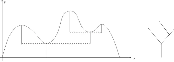
The coding of a compact real tree by a continuous function is now well known and is a key tool for defining random real trees. We consider a continuous functiong : [0,+∞) −→ [0,+∞) with compact support and such that g(0) = 0. We also assume that g is not identically 0. For every 0≤s≤t, we set
mg(s, t) = inf u∈[s,t]g(u),
and
dg(s, t) =g(s) +g(t)−2mg(s, t).
We then introduce the equivalence relation s ∼t if and only if dg(s, t) = 0. Let Tg be the
quotient space [0,+∞)/ ∼. It is easy to check that dg induces a distance on Tg. Moreover,
(Tg, dg) is a compact real tree (see [18], Theorem 2.1). We say thatg is the height process of
the treeTg.
g
s
Figure 1. A height processg and its associated real tree
In order to define a random tree, instead of taking a tree-valued random variable (which implies defining a σ-field on the set of real trees), it suffices to take a continuous stochastic process for g. For instance, wheng is a normalized Brownian excursion, the associated real tree is Aldous’ CRT [9]. We present now how we can define a height process that codes a random real trees describing the genealogy of a (sub)critical CB with branching mechanism
ψ. This height process is defined via a L´evy process that we first introduce.
3.2. The underlying L´evy process. We assume thatψ given by (2) is (sub)critical, i.e. (23) α :=ψ′(0) = ˜α−
Z
(1,+∞)
ℓ π(dℓ)≥0
and that
(24) β >0 and
Z
(0,1)
We consider aR-valued L´evy processX= (Xt, t≥0) with no negative jumps, starting from
0 and with Laplace exponent ψ under the probability measure Pψ: for λ≥0 Eψhe−λXti= etψ(λ). By assumption (24),X is of infinite variation Pψ-a.s.
We introduce some processes related toX. LetJ ={s≥0;Xs6=Xs−}be the set of jump
times ofX. Fors∈ J, we denote by
∆s=Xs−Xs−
the size of the jump of X at time s and ∆s = 0 otherwise. Let I = (It, t ≥ 0) be the
infimum process of X, It = inf0≤s≤tXs, and let S = (St, t ≥0) be the supremum process,
St= sup0≤s≤tXs. We will also consider for every 0≤s≤t the infimum ofX over [s, t]:
Its = inf
s≤r≤tXr.
The point 0 is regular for the Markov processX−I, and−I is the local time ofX−I at 0 (see [12], chap. VII). Let Nψ be the associated excursion measure of the processX−I away
from 0. Letσ= inf{t >0;Xt−It= 0}be the length of the excursion ofX−I underNψ (we
shall see after Proposition 3.7 that the notation σ is consistent with (17)). By assumption (24), we have X0 =I0 = 0 Nψ-a.e.
Since X is of infinite variation, 0 is also regular for the Markov processS−X. The local time, L= (Lt, t≥0), of S−X at 0 will be normalized so that
Eψ[e−λSL−t1] = e−tψ(λ)/λ,
whereL−t1 = inf{s≥0;Ls≥t}(see also [12] Theorem VII.4 (ii)).
3.3. The height process and the L´evy CRT. For each t ≥0, we consider the reversed process at timet, ˆX(t) = ( ˆXs(t),0≤s≤t) by:
ˆ
Xs(t)=Xt−X(t−s)− if 0≤s < t,
and ˆXt(t) =Xt. The two processes ( ˆXs(t),0≤s≤t) and (Xs,0 ≤s≤t) have the same law.
Let ˆS(t) be the supremum process of ˆX(t) and ˆL(t) be the local time at 0 of ˆS(t)−Xˆ(t) with the same normalization asL.
Definition 3.2. ([17], Definition 1.2.1)
There exists a lower semi-continuous modification of the process ( ˆL(t), t≥0). We denote by (Ht, t≥0) this modification.
We can also define this processH by approximation: it is a modification of the process
(25) Ht0 = lim inf
ε→0
1
ε Z t
0
1{Xs<Its+ε}ds.
(see [17], Lemma 1.1.3). In general, H takes its values in [0,+∞], but we have that, a.s. for everyt≥0,
• Hs<+∞ for everys < t such thatXs−≤Its,
• Ht<+∞ if ∆Xt>0
(see [17], Lemma 1.2.1).
We use this process to define a random real-tree that we call the ψ-L´evy CRT via the procedure described above. We will see that this CRT does represent the genealogy of a
3.4. The exploration process. The height process is not Markov in general. But it is a very simple function of a measure-valued Markov process, the so-called exploration process.
If E is a locally compact polish space, let B(E) (resp. B+(E)) be the set of real-valued
measurable (resp. and non-negative) functions defined onE endowed with its Borel σ-field, and let M(E) (resp. Mf(E)) be the set of σ-finite (resp. finite) measures on E, endowed
with the topology of vague (resp. weak) convergence. For any measure µ ∈ M(E) and
f ∈ B+(E), we write
hµ, fi=
Z
E
f(x)µ(dx).
The exploration process ρ = (ρt, t ≥ 0) is a Mf(R+)-valued process defined as follows:
for every f ∈ B+(R+), hρt, fi = R[0,t]dsItsf(Hs) (where dsIts denotes the Lebesgue-Stieljes
integral with respect to the non-decreasing maps7→Its), or equivalently
(26) ρt(dr) =
X
0<s≤t
Xs−<Its
(Its−Xs−)δHs(dr) +β1[0,Ht](r)dr.
In particular, the total mass of ρt ishρt,1i=Xt−It.
Recall (9) and set by conventionH(0) = 0.
Proposition 3.3 ([17], Lemma 1.2.2 and formula (1.12)). Almost surely, for every t >0, • H(ρt) =Ht,
• ρt= 0 if and only if Ht= 0,
• if ρt6= 0, then Suppρt= [0, Ht].
• ρt=ρt−+ ∆tδHt, where ∆t= 0 if t6∈ J.
In the definition of the exploration process, asXstarts from 0, we haveρ0= 0 a.s. To state
the Markov property of ρ, we must first define the process ρ started at any initial measure
µ∈ Mf(R+).
Fora∈[0,hµ,1i], we define the erased measure kaµby
kaµ([0, r]) =µ([0, r])∧(hµ,1i −a), forr ≥0.
Ifa >hµ,1i, we set kaµ= 0. In other words, the measure kaµis the measure µ erased by a
massabackward fromH(µ).
For ν, µ ∈ Mf(R+), and µ with compact support, we define the concatenation [µ, ν] ∈
Mf(R+) of the two measures by:
[µ, ν], f
= µ, f
+
ν, f(H(µ) +·)
, f ∈ B+(R+).
Finally, we set for every µ ∈ Mf(R+) and every t > 0, ρµt =
k−Itµ, ρt]. We say that (ρµt, t≥0) is the processρ started at ρµ0 =µ. Unless there is an ambiguity, we shall write ρt
forρµt. Unless it is stated otherwise, we assume that ρ is started at 0.
Proposition 3.4([17], Proposition 1.2.3). The process(ρt, t≥0)is a c`ad-l`ag strong Markov
process inMf(R+).
Remark 3.5. From the construction of ρ, we get that a.s. ρt= 0 if and only if −It≥ hρ0,1i
and Xt−It= 0. This implies that 0 is also a regular point forρ. Notice thatNψ is also the
excursion measure of the process ρ away from 0, and that σ, the length of the excursion, is
3.5. Notations. We consider the set D of c`ad-l`ag processes in Mf(R+), endowed with the
Skorohod topology and the Borel σ-field. In what follows, we denote by ρ = (ρt, t ≥0) the
canonical process on this set. We still denote byPψ the probability measure on Dsuch that
the canonical process is distributed as the exploration process associated with the branching mechanismψ, and by Nψ the corresponding excursion measure.
3.6. Local time of the height process. The local time of the height process is defined through the next result.
Proposition 3.6([17], Lemma 1.3.2 and Proposition 1.3.3). There exists a jointly measurable process (Las, a≥0, s≥0) which is continuous and non-decreasing in the variablessuch that:
• The occupation time formula holds: for any non-negative measurable function g on
R+ and any s≥0,
why the ψ-L´evy CRT can be viewed as the genalogical tree of aψ-CB.
Proposition 3.7 ([17], Theorem 1.4.1). The process (LaTx, a≥0) is distributed under Pψ as
The occupation time formula implies that
(28) σ(ρ) =
Z +∞
0
Zada,
which is consistent with notation (17). When there is no confusion, we shall writeσ forσ(ρ). We callσ(ρ) the total mass of the CRT as it represents the total population of the associated CB.
Exponential formula for the Poisson point process of jumps of the inverse subordinator of −I gives (see also the beginning of Section 3.2.2. [17]) that for λ >0
(29) Nψh1−e−λσi=ψ−1(λ).
We also recall Lemma 1.6 of [1].
Lemma 3.8. Letθ > 0. The excursion measureNψθ is absolutely continuous w.r.t. Nψ with density e−ψ(θ)σ: for any non-negative measurable function F on the space of excursions, we have
Nψθ[F(ρ)] =Nψ
h
We recall the Poisson representation of Pψx based on the excursion measure Nψ. Let
(˜αi,β˜i)i∈I˜be the excursion intervals ofρ away from 0. For every i∈I˜,t≥0, we set
˜
ρ(i)t =ρ(˜α
i+t)∧β˜i.
We deduce from Lemma 4.2.4 of [17] the following lemma.
Lemma 3.9. The point measure X
i∈I˜
δρ˜(i)(dµ) is under Pψx a Poisson measure with intensity
xNψ(dµ).
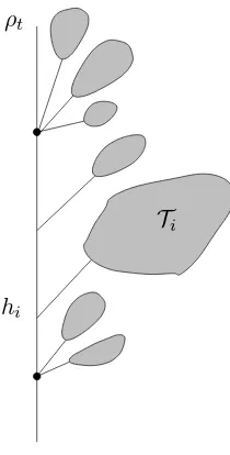
To better understand the links between the L´evy CRT and the exploration process, we can combine the Markov property with the other Poisson decomposition of [17], Lemma 4.2.4. Informally speaking, the measureρtis a measure placed on the ancestral line of the individual
labelled t which describes how the sub-trees “on the right” of t(i.e. containing individuals
s≥t) are grafted along that ancestral line. More precisely, if we denote (Ti)i∈I the family
of these subtrees and we set hi the height where the subtreeTi branches from the ancestral
line oft, then the family (hi,Ii)i∈I givenρtis distributed as the atoms of a Poisson measure
with intensityρt(dh)Nψ[dT].
ρt
hi
Ti
Figure 2. The measureρt and the family (hi,Ii)i∈I
As the mesure Nψ is an infinite measure, we see that the branching points along the
ancestral line of tare of two types:
• binary nodes (i.e. vertex of degree 3) which are given by the regular part of ρt,
• infinite nodes (i.e. vertex of infinite degree) which are given by the atomic part of ρt.
By the definition ofρt, we see that these infinite nodes are associated with the jumps of the
L´evy process X. If such a node corresponds to a jump time s ofX, we call ∆Xs the size of
3.7. The dual process and representation formula. We shall need theMf(R+)-valued
processη= (ηt, t≥0) defined by
(30) ηt(dr) =
X
0<s≤t
Xs−<Its
(Xs−Its)δHs(dr) +β1[0,Ht](r)dr.
The process η is the dual process of ρ under Nψ (see Corollary 3.1.6 in [17]). It represents
how the trees “on the left” oftbranch along the aqncestral line of t.
We recall the Poisson representation of (ρ, η) under Nψ. Let N(dx dℓ du) be a Poisson
point measure on [0,+∞)3 with intensity
dx ℓπ(dℓ)1[0,1](u)du.
For every a > 0, let us denote by Mψa the law of the pair (µa, νa) of measures on R+ with
finite mass defined by: for anyf ∈ B+(R+)
hµa, fi=
Z
N(dx dℓ du)1[0,a](x)uℓf(x) +β Z a
0
f(x)dx,
(31)
hνa, fi=
Z
N(dx dℓ du)1[0,a](x)ℓ(1−u)f(x) +β Z a
0
f(x)dx.
(32)
Remark 3.10. In particularµa(dr) +νa(dr) is defined as 1[0,a](r)drWr, whereW is a
subor-dinator with Laplace exponentψ′−α whereα=ψ′(0) is defined by (23).
We finally setMψ =R+∞
0 da e−αaM ψ a.
Proposition 3.11 ([17], Proposition 3.1.3). For every non-negative measurable function F
on Mf(R+)2,
Nψ Z σ
0
F(ρt, ηt)dt
=
Z
Mψ(dµ dν)F(µ, ν),
where σ = inf{s >0;ρs= 0} denotes the length of the excursion.
4. Super-critical L´evy continuum random tree
We shall construct a L´evy CRT with super-critical branching mechanism using a Girsanov formula.
Let ˜ψ be a (sub)critical branching mechanism. The process Z = (Za, a ≥ 0), where
Za =LaTx, is a CB with branching mechanism ˜ψ. We have P
˜ ψ
x-a.s. Z∞ = lima→+∞Za = 0.
We shall call x the initial mass of the ˜ψ-CRT under Pψx˜. Formula (28) readily implies the
following Girsanov formula: for any non-negative measurable function F, and q ≥0,
(33) Eψ˜
x
h
M∞ψ,q˜ F(ρ)i=Eψ˜q
x [F(ρ)],
whereM∞ψ,q˜ is given by (21).
We will use a similar formula (with q <0) to define the exploration process for a super-critical L´evy CRT with branching mechanism ψ. Because super-critical branching process may have an infinite mass, we shall cut it at a given level to construct the corresponding genealogical continuum random tree, see [16] whenπ = 0.
For a ≥ 0, let Ma
f = Mf([0, a]) be the set of non-negative measures on [0, a] and let
Da be the set of c`ad-l`ag Ma
f-valued process defined on [0,+∞) endowed with the Skorohod
topology. We now define a projection from D to Da. For ρ = (ρ
the time spent below levelaup to timet: Γρ,a(t) =R0t1{H(ρs)≤a} dsand its right continuous
with the convention ρ+∞= 0. By construction we have the following compatibility relation:
πa◦πb=πa for 0≤a≤b.
Let ψ be a super-critical branching mechanism which we suppose to be conservative, i.e. (3) holds. Recall q∗ is the unique (positive) root of ψ′(q) = 0. In particular the branching mechanismψq is critical if q =q∗ and sub-critical if q > q∗.
We consider the filtration H= (Ha, a≥0) where Ha is the σ-field generated by the c`
ad-l`ag process πa(ρ) and the class of P ψq∗
x negligible sets. Thanks to the second statement of
Proposition 3.6, we get thatZ isH-adapted. Furthermore the proof of Theorem 1.4.1 in [17] yields thatZ is a Markov process w.r.t. the filtrationH. In particular the process Mψq∗,−q∗ defined by (8) is thanks to Theorem 2.2 aH-martingale under Pψxq∗.
Letq ≥q∗. We define the distributionPxψ,a (resp. Nψ,a) of the ψ-CRT cut at level awith
initial mass x, as the distribution of πa(ρ) under Maψq,−qdPψxq (resp. eqZa+ψ(q)
Ra
0 ZrdrdNψq): for any measurable non-negative functionF,
Exψ,a[F(ρ)] =EψxqhMaψq,−qF(πa(ρ))i,
Proof. Let q > q∗. For any non-negative measurable functionF, we have
Eψq
Excursion theory then gives the result for the excursion measures.
Proposition 4.2. Let (ρa, a ≥ 0) be the canonical process on W. There exists a probabil-ity measure P¯ψx (resp. an excursion measure N¯ψ) on W, such that, for every a ≥ 0, the
distribution of ρa underP¯ψx (resp. N¯ψ) is Pψ,ax (resp. Nψ,a) and such that, for 0≤a≤b
(38) πa(ρb) =ρa P¯ψx-a.s. (resp. N¯ψ-a.e.).
Proof. To prove the existence of such a projective limit, it is enough to check the compatibility relation betweenPψ,bx and Pψ,ax for everyb≥a≥0.
Let 0≤a≤b. We get
Eψ,b
x [F(πa(ρ))] =Eψq ∗ x
h
Mψq∗,−q∗
b F(πa◦πb(ρ))
i
=Eψq∗
x
h
Mψq∗,−q∗
b F(πa(ρ))
i
=Eψxq∗ h
Mψq∗,−q∗
a F(πa(ρ))
i
=Eψ,ax [F(ρ)],
where we used the compatibility relation of the projectors for the second equality and the fact thatMψq∗,−q∗ is aH-martingale for the third equality. We deduce that Pψ,bx ◦πa=Pψ,ax .
This compatibility relation implies the existence of a projective limit ¯Pψx. The result is
similar for the excursion measure.
Let us remark that the definitions of ¯Pψx and ¯Nψ are also valid for a (sub)critical branching
mechanismψ, with the convention q∗ = 0. In particular, we get the following corollary.
Corollary 4.3. If ψ is (sub)critical, then the law of the process (πa(ρ), a ≥ 0) under Pψx
(resp. Nψ) is P¯ψx (resp. N¯ψ).
By construction the local time at levela of ρb forb≥adoes not depend on b, we denote by Zaits value. Property (ii) of Theorem 2.2 implies that Z = (Za, a≥0) is under ¯Pψx a CB
with branching mechanismψ. Hence, the probability measure ¯Pψx can be seen as the law of the exploration process that codes the super-critical CRT associated with ψ.
We get the following direct consequence of Properties (i) and (ii) of Lemma 2.4 and of the theory of excursion measures.
Corollary 4.4. Letq >0such thatψ(q)≥0. Then, the probability measureP¯ψxq is absolutely
continuous with respect to P¯ψx with
dP¯ψq
x
dP¯ψx =M
ψ,q
∞ = eqx−ψ(q)σ1{σ<+∞}.
The measure N¯ψq is absolutely continuous with respect to N¯ψ with
dN¯ψq
dN¯ψ = e− ψ(q)σ1
{σ<+∞}.
If the total mass ofZ,σ=R+∞
0 Zada, is finite, thenρais the projection of a well defined
exploration process.
Lemma 4.5. On {σ < +∞}, there exists ρ∞ ∈ D such that ρa = πa(ρ∞) for all a ≥ 0,
¯
Proof. It is enough to get the result under ¯Pψx.
First we assume that ψ is (sub)critical. Proposition 3.6 implies that Rt
01{H(ρs)≤a} ds increases tot asagoes to infinity. Using (34), (35) and the right continuity of ρ, we deduce thatPψx-a.s. for allt≥0, lim
The caseψ super-critical is then a consequence of Corollary 4.4.
Without confusion, we shall always writePψ instead of ¯Pψ and Nψ instead of ¯Nψ and call
them the law or the excursion measure of the exploration process of the CRT, whetherψ is super-critical or (sub)critical. And we shall writeρfor the projective limit (ρa, a≥0) onW,
and make the identification ρ = ρ∞ ∈ D when the latter exists that is when σ defined by (28) is finite.
Recallψ−1is given by (18). We now extend formula (29) for general branching mechanism.
Lemma 4.6. Let σ be given by (28). We have for λ≥0:
where we used (36) for the first equality, (8) for the second, Lemma 3.9 for the third, (37) for the fifth, and (1) of Theorem 2.2 for the last. We then let agoes to infinity to get the first equality of the lemma, and use (20) to get the second.
5. Pruning
We keep notations from Section 3. Recall that D is the set of c`ad-l`ag Mf(R+)-valued
process, andW is the set ofD-valued processes. LetR= (ρθ, θ≥0) be the canonical process
on W.
Let ψ be a (sub)critical branching mechanism. The pruning procedure developed in [6] whenπ = 0, [1] whenβ= 0 and in [5] or [25] for the general case, yields a probability measure onW, ˜Pψx, such thatR is Markov and the law ρθ under ˜Pψx is Pψθ
x for all θ≥0. Furthermore
ρθ codes for a sub-tree ofρθ′
if θ≥θ′. We recall the construction of ˜Pψx in Section 5.1.
appears at a random time. At timeθ, we remove all the vertex of the initial tree that contains a mark on their lineage. In terms of exploration processes, we get ρθ by a time change of
the processρthat skips all the times trepresenting individuals that received a mark on their lineage by timeθ. We explain more precisely the pruning procedure.
5.1.1. Marks on the nodes. Let (Xt, t ≥0) be the L´evy process with branching mechanism
ψ and letρ be the corresponding exploration process. Recall (∆s, s∈ J) denotes the set of
jumps ofX. Conditionally on X, we consider a family
(Ts, s∈ J)
of independent exponential random variables with respective parameter ∆s. We define the
M(R2+)-valued process M(nod)= (Mt(nod), t≥0) by
Mt(nod)(dr, dv) = X
0<s≤t
Xs−<Ist
δTs(dv)δHs(dr).
For fixedθ≥0, we will consider theM(R+)-valued process M(nod)
t (dr,[0, θ]) whose atoms
give the marked nodes : each node of infinite degree is marked independently from the others with probability 1−e−θ∆s where ∆
s is the mass (i.e. the height of the jump) associated with
the node.
Remark 5.1. Although different from the measure process that defines the marks on the nodes in [1] (formula (12)), this construction gives the same marks (see Introduction of [1]).
Remark 5.2. The time parameter introduced here allows to construct a coherent family of marks. Indeed, for θ′ > θ, the atoms of Mt(nod)(dr,[0, θ]) are still atoms ofMt(nod)(dr,[0, θ′]). In other words, there are more and more marked nodes as θ increases, which allows to construct a ’decreasing’ tree-valued process in Section 5.1.3.
5.1.2. Marks on the skeleton. Let M(ske) = (Mt(ske), t≥0) be a L´evy snake with lifetimeH
and spatial motion a Poisson point process with intensity
2β1{u>0}du.
(See [17] for the definition of a L´evy snake and [5] for the extension to a discontinuous height processH, see also [25]).
In other words, M(ske) is a M(R2+)-valued process such that, conditionally on the
explo-ration processρ,
• For every t≥0,Mt(ske)(dr, du) is a Poisson point measure with intensity
2β1[0,Ht](r)dr1{u>0}du, • For every 0≤t≤t′, withHt,t′ := inf
s∈[t,t′]Hs, then: – The measures Mt(ske)(dr, du)1r∈[0,H
t,t′] and M
(ske)
t′ (dr, du)1r∈[0,H
t,t′] are equal,
– The random measures Mt(ske)(dr, du)1r∈[Ht,t′,Ht] and M
(ske)
t′ (dr, du)1r∈[Ht,t′,Ht′]
5.1.3. Definition of the pruned processes. We define the mark process as
(39) M(mark) =M(nod)+M(ske).
The process ((ρt, Mt(mark)), t≥0) is called the marked exploration process. It is Markovian,
see [25] for its properties. We denote by ˆPψx its law and by ˆNψ the corresponding excursion
measure.
For everyθ >0 and t >0, we set
m(θ)t =Mt(mark) [0, Ht]×[0, θ]
.
The random variable m(θ)t is the number of marks at time θ that lay on the lineage of the individual labeled byt. We will only consider the individuals without marks on their lineage. Therefore, we set
(40) A(θ)t =
Z t
0 1
{m(sθ)=0}ds and C
(θ)
t = inf{r ≥0;A(θ)r ≥t}
its right-continuous inverse. Finally, we defineρθ = (ρθt, t≥0),M(mark),θ = (Mt(mark),θ, t≥0) by
ρθt =ρ
Ct(θ)
,
Mt(mark),θ([0, h]×[0, q]) =M(mark)
Ct(θ) ([0, h]×(θ, q+θ]).
We shall use in Section 7 the pruning operator Λθ defined on the marked exploration
process by
(41) Λθ(ρ, M(mark)) = (ρθ, M(mark),θ).
Using the lack of memory of the exponential random variables and of properties of Poisson point measure, it is easy to get that
Lemma 5.3. The process R= (ρθ, θ≥0) is Markov.
The W-valued process R codes for a decreasing family of CRT, which we shall call a
ψ-family of pruned CRT. A direct application of Theorem 1.1 of [5] gives the marginal dis-tribution.
Proposition 5.4. The marked exploration process (ρθ, M(mark),θ) under Pψx (resp. Nψ) is
distributed as (ρ, M(mark)) underPψθ
x (resp. Nψθ).
We shall now concentrate on the process R. Let ˜Pψx be the law of R and ˜Nψ be the
corresponding excursion measure.
We deduce the following compatibility relation from the Markov property ofRand Propo-sition 5.4.
Corollary 5.5. Let θ0 ≥ 0. The law under P˜ψx (resp. N˜ψ) of the process (ρθ0+θ, θ ≥ 0) is
˜
Pψθ0
x (resp. N˜ψθ).
{s ≥ 0, m(θ)s = 0} and write O =
[
i∈I
(αi, βi). For every i ∈ I, we define the exploration
processρ(i) by: for everyf ∈ B+(R+), t≥0,
hρ(i)t , fi=
Z
[Hαi,+∞)
f(x−Hαi)ρ(αi+t)∧βi(dx).
We have the following theorem.
Theorem 5.6 (Special Markov Property). Let θ > 0 and let (Zθ
t, t≥0) be the CSBP coded
by ρθ. The point measure
X
i∈I
δ(H
αi,ρ(i))(dh, dµ)
underPψx (or Nψ) conditionally given(ρθ
t, t≥0), is a Poisson point measure of intensity
1[0,+∞)(h)Zhθ dh 2βθNψ(dµ) + Z
(0,+∞)
π(dr)(1−e−θr)Pψ
r(dµ)
!
.
This theorem describes in fact the joint law of (ρ(θ), ρ(θ′)
) forθ < θ′and hence the transition
probabilities of the processRand of the time-reversed process. In terms of trees, by definition, the treeT(θ′)
is obtained from the tree T(θ) by pruning it with the pruning operator Λ θ′−θ.
Conversely, to get the treeT(θ) from the treeT(θ′)
, we pick some individuals of the treeT(θ′)
according to a Poisson point measure and add at these points either a L´evy tree associated with the branching mechanismψθ (first part of the intensity of the Poisson measure), or an
infinite node of sizer and trees distributed asPψθ
r (second part of the intensity of the Poisson
measure).
5.2. Pruning of super-critical CRT. We now use the same Girsanov techniques of Section 4 to define aψ-family of pruned CRT whenψis super-critical.
Let ψ be a super-critical branching mechanism which we suppose to be conservative, i.e. (3) holds. Recall q∗ is the unique (positive) root of ψ′(q) = 0. In particular the branching mechanismψq is critical if q =q∗ and sub-critical if q > q∗.
Letq ≥q∗. LetR= (ρθ, θ≥0) be the canonical process onW. We setZ = (La∞(ρ0), a≥0) which is under ˜Pψxq(dR) a CB with branching mechanismψq. The processZis also well defined
under the excursion measure ˜Nψq(dR). We write π
a(R) = (πa(ρθ), θ≥0). Notice that given
the marks (i.e. givenM(nod) and M(ske)), we have πa(ρθ) = (πa(ρ))θ.
Leta≥0. We define the distribution ˜Pψ,ax (resp. excursion measure ˜Nψ,a) of aψ-family of
pruned CRT cut at levelawith initial massx, as the distribution ofπa(R) underMaψq,−qd˜Pψxq
(resp. eqZa+ψ(q)R0aZrdrdN˜ψq): for any measurable non-negative functionF, we have: ˜
Pψ,ax [F(R)] = ˜Pψxq h
Mψq,−q
a F(πa(R))
i
and
˜
Nψ,a[F(ρ)] = ˜NψqheqZa+ψ(q)R0aZrdrF(π
a(ρ))
i .
Same arguments as for Lemma 4.1 give the following result.
Lemma 5.7. The distributions P˜ψ,ax andN˜ψ,a do not depend on the choice of q≥q∗.
As in Section 4, see Proposition 4.2, the families of measures (˜Pψ,ax , x≥0) and ( ˜Nψ,a, a≥0)
• For every a≥0, Ra is distributed as ˜Pψ,ax ,
• For every a < b,πa(Rb) =Ra.
We write ˜Pψx for the distribution of this projective limit and ˜Nψ for the corresponding
excur-sion measure.
By construction the local time at levelaofπb(ρθ) forb≥adoes not depend onb, we denote
byZaθits value. Proposition 5.4 and Property (ii) of Theorem 2.2 imply thatZθ = (Zaθ, a≥0) is under ˜Pψx a CB with branching mechanism ψθ started at x. Following (28), we define σθ =R0∞Zaθda. And, when there is no confusion, we write σ forσ0.
Following Corollaries 4.3, 4.4 and Lemma 4.5, we easily get the following theorem.
Theorem 5.8. Letψ be a conservative branching mechanism. Let(Ra, a≥0) be aW-valued
process under P˜ψx (resp. N˜ψ).
(1) Ifψis (sub)critical, then(Ra, a≥0)underP˜xψis distributed as((πa(ρθ), θ≥0), a≥0)
under Pψx.
(2) Let q >0 such that ψ(q)≥0. Then, the probability measureP˜ψq
x is absolutely
contin-uous with respect to P˜ψx with
dP˜ψxq dP˜ψx =M
ψ,q
∞ = eqx−ψ(q)σ1{σ<+∞}.
The measure N˜ψq is absolutely continuous with respect to N˜ψ with
dN˜ψq
dN˜ψ = e
−ψ(q)σ1
{σ<+∞}.
(3) On {σ <+∞}, there exists R∞ ∈ W such that Ra=πa(R∞) for all a≥0, ˜Pψx-a.s.
or N˜ψ-a.e.
Without confusion, we shall always writePψ instead of ˜Pψ and Nψ instead of ˜Nψ and call
them the law or the excursion measure ofψ-pruned family of exploration processes, whether
ψ is super-critical or (sub)critical. Theψ-pruned family of exploration processes codes for a
ψ-pruned family of continuum random sub-trees.
And we shall write (ρθ, θ ≥ 0) for the projective limit (Ra, a ≥ 0), and identify it with
R∞ ∈ W when the latter exists, that is when σ defined by (28) is finite. Notice that if σθ is
finite then the exploration processρθ codes for a CRT with finite mass.
5.3. Properties of the branching mechanism. Let ψ be a branching mechanism with parameter (α, β, π). Let Θ′ be the set of θ∈Rsuch that
(42)
Z
(1,+∞)
e−θℓπ(dℓ)<+∞.
We setθ∞= inf Θ′. Notice that we have either Θ′ = [θ∞,+∞) or Θ′ = (θ∞,+∞) and that
θ∞≤0. Notice thatψθ exists for everyθ∈Θ′ and is conservative for everyθ > θ∞. We set
Θ ={θ∈Θ′;ψθ is conservative}. Notice that Θ⊂Θ′⊂Θ∪ {θ∞}.
For instance, we have the following examples of critical branching mechanisms: i) Quadratic case: ψ(u) =βu2, Θ = Θ′=R.
ii) Stable case: ψ(u) =cuα with α∈(1,2), Θ = Θ′ = [0,+∞).
iii) ψ(u) = (u+ e−1) log(u+ e−1) + e−1: Θ = Θ′ = [−e−1,+∞). (Notice that ψθ∞(u) =
iv) ψ(u) = u−1 + 1+u1 is associated with (˜α, β, π) where ˜α = 2/e, β = 0 and π(dℓ) = e−ℓ1{ℓ>0}dℓ: Θ = Θ′ = (−1,+∞).
For the end of this subsection, we assume that ψis CRITICAL and that β >0 or π 6= 0. Remark thatψis a one-to-one function from [0,+∞) onto [0,+∞) and we denote byψ−1 its
inverse function. For θ <0 such that θ ∈ Θ′, we define ¯θ = ψ−1(ψ(θ)) or equivalently ¯θ is the unique positive real number such that
(43) ψ(¯θ) =ψ(θ).
Since ψis continuous and strictly convex, if θ∞∈Θ′, we have
(44) θ¯∞= lim
θ↓θ∞
¯
θ.
Notice that in this case ¯θ∞ is finite. Ifθ∞6∈Θ′, we define ¯θ∞ using (44).
Lemma 5.9. Let ψ be CRITICAL with parameters (˜α, β, π) such that β >0 or π 6= 0. If
θ∞6∈Θ′ then θ¯∞= +∞.
Proof. We assume that θ∞ 6∈ Θ′. It is enough to check that limθ↓θ∞ψ(θ) = +∞ to get
¯
θ∞= +∞.
We first consider the caseθ∞=−∞. Sinceψ′(0) = 0 andψis strictly convex, we get that limθ↓θ∞ψ(θ) = +∞.
Ifθ∞>−∞, then using that (42) does not hold forθ∞and monotone convergence theorem,
we get that limθ↓θ∞ψ(θ) = +∞.
6. A tree-valued process
Letψ be a branching mechanism. We assumeθ∞<0. We write Rq= (ργ+q, γ≥0).
We deduce from Corollary 5.5 that the families of measures (Pψθ, θ∈Θ) and (Nψθ, θ∈Θ) satisfy the following compatibility property: if θ′ < θ,θ′ ∈Θ, the process Rθ−θ′ underPψθ′
(resp. Nψθ′) is distributed as R
0 underPψθ (resp. Nψθ).
Hence, there exists a projective limit R = (ργ, γ ∈ Θ) such that, for every θ ∈ Θ, the process (ρθ+γ, γ≥0) is distributed as (ργ, γ≥0) underPψθ. We denote byPPPψ the distribution of the projective limitR, and byNNNψ the corresponding excursion measure. We still writeRθ
for (ρθ+γ, γ≥0) for all θ∈Θ.
The process R = (ρθ, θ ∈ Θ) is Markovian, thanks to Lemma 5.3. It codes for a tree-valued Markov process, which evolves according to a pruning procedure. At time θ, ρθ has distribution Pψθ. Recall σ
θ is the mass of the CRT coded by ρθ. It is not difficult to check
that Σ = (σθ, θ ∈ Θ) is a non-increasing Markov process taking values in [0,+∞] and we
shall consider a version of R such that the process Σ is c`ad-l`ag. From the continuity of ψ, we deduce that the Laplace transform of σθ given in Lemma 4.6 is continuous, and thus the
process Σ is continuous in probability.
See [15] for the distribution of the decreasing rearrangement of the jumps of (σθ, θ≥0) in
the case of stable trees. We deduce from the pruning procedure that a.s. limθ→+∞σθ = 0.
Notice that by considering the time returned process (ρ−θ, θ < θ∞), we get a Markovian family of exploration processes coding for a family of increasing CRTs.
Remark 6.1. Recall q∗ is the unique root of ψ′(q) = 0 and thatψq∗ is critical. Using a shift
onθbyq∗, that is replacingψbyψq∗, one sees that it is enough, when studyingR, to assume
Lemma 6.2. Let ψ be a critical branching mechanism with parameter (α, β, π). For any
θ ∈ Θ, and any non-negative measurable function F defined on the state space of R0, we
have
(45) NNNψ
F(Rθ)1{σθ<∞}
=NNNψθ
F(R0)1{σ0<∞}
=NNNψhF(R0) e−ψ(θ)σ0i.
Proof. The first equality is just the ’compatibility property’ stated at the beginning of this section.
Forθ≥0, the second equality is a direct consequence of (ii) from Theorem 5.8.
Forθ <0, let q= ¯θ−θ. Notice that ψθ(q) =ψ(¯θ)−ψ(q) = 0 and (ψθ)q=ψθ¯. We deduce
from (ii) of Theorem 5.8 that
N
NNψθ¯[F(R
0)] =NNNψθ
F(R0)1{σ0<∞}
.
Since ¯θ >0 andψ(θ) =ψ(¯θ), we get from (2) of Theorem 5.8 that
N N
Nψθ¯[F(R
0)] =NNNψ
h
F(R0) e−ψ(¯θ)σ0
i
=NNNψ h
F(R0) e−ψ(θ)σ0
i .
This ends the proof.
We deduce directly from this lemma the following result on the conditional distribution of the exploration process knowing the total mass of the CRT.
Corollary 6.3. Let ψ be a branching mechanism with parameter (α, β, π) such that (42) holds. The distribution of(ρθ+γ, γ≥0) conditionally on{σθ=r}does not depend on θ∈Θ.
We assume from now-on that ψ is CRITICAL and that θ∞ <0. The first assumption is not restrictive thanks to Remark 6.1.
Notice that ρθ codes for a critical (resp. sub-critical, resp. super-critical) CRT if θ = 0
(resp. θ >0, resp. θ <0). In particular, we have σθ <+∞ a.s. ifθ≥0.
We consider the explosion time
A= inf{θ∈Θ, σθ<+∞},
with the convention that inf∅ = θ∞. In particular, we have A ≤ 0 PPPψ
x-a.s. and NNNψ-a.e.
Moreover, since the process (σθ, θ∈Θ) is c`ad-l`ag, we have, on{A > θ∞},σθ = +∞for every
θ < Aand σθ <+∞ for every θ > A. For the time reversed process, A is the random time
at which the tree gets an infinite mass.
We first give a lemma on the conditional distribution ofσ.
Lemma 6.4. Let q∈Θ, q≤θ. We have, for λ≥0,
NNNψ[e−λσq|ρθ] = e−σθψθ(ψq−1(λ))
andNNNψ[σq<+∞|ρθ] = e−σθψθ(¯q−q), where q¯=ψ−1(ψ(q)).
Proof. Let λ >0 and F be a non-negative measurable function defined onW. We write Zaq
for the local time at levelaof the exploration process ρq. Using (17), we have
(46) NNNψ[e−λσqF(ρθ)] = lim
a→∞N
NNψ[e−λ
Ra
0 Z q
r drF(ρθ)].
We set
Ia=NNNψ[e−λ
Ra
0 Z q
LetG(πa(ρθ)) =EEEψ[F(ρθ)|πa(ρθ)]. We have, withθ′=θ−q≥0,
where for the first equality we conditioned with respect toσ(πa(ρq)), used Girsanov formula
for the third equality and Theorem 5.6 for the last equality with
Kha= 2βθ′Nψ
Using again Theorem 5.6 and Girsanov formula, we get
Ia=NNNψ[e−qZ
Notice also that, thanks to Girsanov formula,
˜
We deduce from (46) and (47), that
The next theorem gives the distribution of the explosion time A under the measureNNNψ.
Recall the definition of ¯θin (43) and (44).
Theorem 6.5. We have, for all θ∈[θ∞,+∞),
(48) NNNψ[A > θ] = ¯θ−θ
and
NNNψ[A=θ∞] = (
0 if θ∞6∈Θ′,
+∞ if θ∞∈Θ′.
Proof. We have for all θ > θ∞ N N
Nψ[A > θ] =NNNψ[σθ= +∞]
=Nψθ[σ = +∞]
= lim
λ→0
Nψθh1−e−λσi
= lim
λ→0ψ −1 θ (λ)
=ψθ−1(0),
where we used (4.6) for the fourth equality. We get, fort >0,
ψθ(t) = 0 ⇐⇒ ψ(t+θ) =ψ(θ) ⇐⇒ t+θ= ¯θ,
and thus ψθ−1(0) = ¯θ−θ, which gives the first part of the theorem for θ > θ∞. Making θ
decrease to θ∞ gives the result for θ∞.
For the second part of the theorem, we apply the second assertion of Lemma 6.4 with
θ= 0. We have, for every q≤0,
N N
Nψ[σq<+∞|ρ] = e−σψ(¯q−q).
Then, we have
N N
Nψ[A=θ∞|ρ] =NNNψ[∀q > θ∞, σq<+∞|ρ]
= lim
q→θ∞
NNNψ[σq <+∞|ρ]
= lim
q→θ∞e
−σψ(¯q−q)
=
(
0 if θ∞6∈Θ′
e−σψ(¯θ∞−θ∞) if θ∞∈Θ′, withψ(¯θ∞−θ∞)<+∞,
where the last equality is a consequence of Lemma 5.9. Then, integrating with respect to ρ
gives the theorem.
Remark 6.6. Sinceψ−1 is smooth, we deduce that the mappingq 7→q¯is differentiable with
dq¯
dq = ψ′(q)
ψ′(¯q)·
Thus, whenθ∞ 6∈Θ, we have that the law of A underNNNψ has a density with respect to the
Lebesgue measure onRgiven by
1{r∈(θ∞,0)}
1−ψ′(r)
ψ′(¯r)
Theorem 6.7. (i) Let θ ∈ (θ∞,0). Under NNNψ, conditionally on {A = θ}, we have for
(ii) If θ∞∈Θ, we have for any non-negative measurable function F
(50) NNNψ
Proof. Let F be a non-negative measurable function defined on the state space of R0. Using
Lemma 6.4, we get for every θ∞< q≤θ <0, Thus, we get that the mapping
q 7→NNNψ[F(Rθ)1{A>q}]
Finally, using thatσ is right continuous, we have
NNNψ[F(RA), A∈dθ] We deduce from Lemma 6.2 that
NNNψ[F(RA)|A=θ] =N This proves (49) but for the normalizing constant. It also implies that
NNNψ[e−λσA|A=θ] = N
ψθ[σe−λσ]
Nψθ[σ1