NGA Workshop Whitepapers

(1)

National Research Council

Workshop on New Research Directions for the

National Geospatial-Intelligence Agency

White Papers

May 17-19, 2010, Workshop National Academies Keck Center

(2)

(3)

Workshop on New Research Directions for the

National Geospatial-Intelligence Agency

White Papers

May 17-19, 2010, Workshop National Academies Keck Center

(4)

(5)

iii

COMMITTEE ON NEW RESEARCH DIRECTIONS FOR THE

NATIONAL GEOSPATIAL-INTELLIGENCE AGENCY

KEITH C. CLARKE, Chair, University of California, Santa Barbara LUC E. ANSELIN, Arizona State University, Tempe

ANNETTE J. KRYGIEL, Independent Consultant, Great Falls, Virginia CAROLYN J. MERRY, Ohio State University, Columbus

SCOTT A. SANDGATHE, University of Washington, Seattle MANI SRIVASTAVA, University of California, Los Angeles

JAMES J. THOMAS, Pacific Northwest National Laboratory, Richland, Washington

National Research Council Staff

ANNE M. LINN, Study Director

LEA A. SHANLEY, Postdoctoral Fellow JASON R. ORTEGO, Research Associate ERIC J. EDKIN, Senior Program Assistant

NOTICE

To set the stage for the May 17-19 workshop, the committee commissioned white papers from leading experts in NGA’s traditional core areas:

 remote sensing and imagery science  photogrammetry and geomatics  geodesy and geophysics

 cartographic science

 geographic information systems and geospatial analysis

(6)

(7)

v

Calibration of the Aerial Photogrammetric System

Dean C. Merchant Geodetic Science Department

Ohio State University

ABSTRACT: A brief history of aerial photogrammetry is presented, which leads to recent applications of modern digital cameras with associated sensors. The concept of measurement system calibration is emphasized since it appears to have potential for greatly improving the geospatial accuracy and reliability of NGA sensors. Although the modern digital mapping camera is emphasized, calibration has a useful role in development of most geospatial sensors. An example of recent results of calibration is provided for an airborne digital camera, the most recent Zeiss airborne digital camera, the RMK-D II. The quality of the result is good with the fit of image residuals at about 2 microns rmse. Based on the quality of these results,

recommendations for calibration research are made in the context of the NGA mission.

Forward

I have been asked to write concerning the areas of photogrammetry and geomatics as they

pertain to the geo-spatial interests of the NGA. Because of my area of interest, I will concentrate on photogrammetry in terms of current capability, potential areas of technical improvements, and future use. Improvements will be framed in the context of NGA’s interests, particularly in terms of timeliness and geo-spatial accuracy.

To begin, I will comment briefly on history of photogrammetry, particularly as it leads to applications of interest to the NGA. This will be followed with comments on the state of the art and the central topic of calibration of measurement systems, particularly of the type used by NGA. All comments are made without benefit of classified information.

BRIEF HISTORY OF PHOTOGRAMMETRY

Most of the early development of photogrammetry was done in Europe during the early part of the 20th century. The theory was well-developed by Otto Von Gruber (1942) and others. The bulk of this early photogrammetric equipment was developed and marketed by Zeiss of

Germany. Of particular interest were their photo theodolites and aerial cameras. Zeiss was also an early developer of the stereo comparator and of map compilation equipment. Other early European developments occurred in France, England, Italy, Austria and Holland.

(16)

2 New Research Directions for the NGA: A Workshop – White Papers

During this early period, Fairchild Camera became the primary producer of aerial mapping cameras. In fact, Fairchild claims to have produced 90% of all aerial cameras, including reconnaissance cameras, used by the Allies during WWII. Cameras were also made by Park Aerial Surveys and Abrams Aerial Surveys. Little map compilation equipment was developed in the US during this early period. Users relied on, for example, the Bausch and Lomb (B&L) copy of the Zeiss Multiplex, a stereoscopic projection type plotting instrument.

Early and mid-history of the developments in photogrammetry are well- documented in the sequence of Manuals of Photogrammetry published by the American Society of Photogrammetry (ASP & ASPRS, 1980).

The term “analytical photogrammetry” evolved as digital methods of computation became available. Much of the credit for advancements both in theory and application of analytical methods in the U.S. belong first to Dr. Hellmut Schmid, then working for the US Army and subsequently the U S Coast and Geodetic Survey. While at the Army Aberdeen Proving Ground, Dr. Schmid guided Dwane Brown in the theory of analytical photogrammetry.

These interests led Brown to work for the US Air Force at the Air Force Missal Test Center (AFMTC) at Patrick AFB. Here, he was instrumental in developing the theory of spatial intersection for tracking test missiles by photo-theodolites. For improved spatial tracking accuracies, Brown adapted the 36 inch focal length lens from the B&L K-38 camera to a ground based camera for tracking. This approach depended on a star-field background to establish angular orientation for a series of widely spaced tracking cameras. With the known locations of these tracking cameras, an extremely accurate tracking by means of photogrammetric

intersection was accomplished.

Brown began to develop his interest in camera calibration with early work conducted in a large hangar at Patrick AFB. By converging three or more cameras focusing on common targets placed on the hangar floor and using other exterior orientation steps, he was able to establish a procedure leading to both exterior and interior orientation for all participating cameras.

Subsequently it was established that only first approximations of target locations were required for a solution of not only camera orientations but also target locations. This aspect of

photogrammetry leads to some extended applications of calibration and target location that may be of interest to the NGA.

Later, then working for Duane Brown and Associates (DBA) and under contract to USAF, Brown demonstrated the internal accuracy of the Fairchild KC-6A camera as being one part in one million of the flying height. This camera, as a part of the USAF USQ-28 Geodetic Sub-System, was flown in the RC-135 aircraft at an altitude of 20,000 feet, augmented by an inertial system, and tracked by ground based ballistic cameras. This experiment clearly established aerial analytical photogrammetry as a reliable geodetic survey tool.

(17)

3 Calibration of the Aerial Photogrammetric System

photogrammetry. Modern digital storage devices, electronic (digital) cameras, and optical scanning devices (LIDAR) are opening opportunities for wider applications for geospatial image collection devices. Rapid response times and higher geospatial accuracies will be some of the directions taken by research to meet the needs of NGA. Central to these developments will be the notion of measurement system calibration.

CONCEPT OF MEASUREMENT SYSTEM CALIBRATION

Common to all NGA image collection systems is the concept of measurement system calibration. During the designing and testing of new measurement systems, it is common practice to simply sum the estimated error contributions of each component to generate an estimated error

representing the system. A more sophisticated approach has been to “cascade” the errors producing a more theoretically correct result. In such cases of error estimation of actual

operating measurement systems, the environment in which the systems operate is neglected. The preferred approach is to assess the system’s operational measurement performance based on comparison of measurements to a standard of higher accuracy. In the aerial case, this is done by comparing independent resected photos to the exposure stations coordinates produced by GPS. In this case, GPS represents the independent standard of higher accuracy. As an alternative, the results of an aerial, bundle block adjustment can be used to produce coordinates for comparison to ground targets as the independent standard. After sufficient comparisons of the “final

product” to its higher accuracy equivalent, the system can be said to have been calibrated by an in situ method. Comparisons of geospatial measurement accuracies based on the laboratory calibration to the in situ methods will be discussed below.

Reference is made to a classic treatment of the concept of measurement system calibration by Churchill Eisenhart (1962) then a member of the staff of the US Bureau of Standards. His complete approach to calibration is ideally suited to the needs of many of the NGA’s various geospatial data collectors. Accordingly, it will be discussed in some detail and serve as a basis for future R&D comments. To summarize Eisenhart’s approach to measurement system calibration, he states that two conditions must be met:

Prepare measurement system specifications. Establish a state of statistical control.

Measurement system specifications fully describe all elements of the measurement system along with appropriate ranges. For the aerial case, elements include the camera, platform, software, and provisions for geodetic control to name a few. As an example of range, the altitude may be specified as between 100 and 1000 meters. Environment can also play a role. Temperature of the camera at collection time can greatly affect the focal length.

(18)

of statistical control. As long as results over time remain within acceptable limits of geospatial accuracy, the operational aerial photogrammetric system is said to be acceptable for application, and continues in a state of calibration.

JUSTIFICATION FOR CALIBRATION

The justification for NGA interest in measurement system calibration rests primarily in their need for geospatial coordinate accuracy. The USAF experiences with results of their USQ-28 project gave early confidence that airborne analytical photogrammetric methods can produce geospatial coordinates considered to be of geodetic quality. As indicated earlier, Brown was able to achieve accuracies approaching one part in one million of the camera flight altitude.

Early work of Goad (1989) indicated the potential for GPS to accurately determine the position of a moving vehicle. At White Sands Proving Ground he measured the track position of a moving sled equipped with GPS. Comparison of the track to the GPS positions produced mm discrepancies of 2 mm rmse.

It was not until GPS evolved to a satisfactory efficiency that it could replace the operationally expensive use of ground based, stellar oriented cameras to position the aerial camera at exposure time. The first well- documented application of use of GPS to position the camera over a

controlled and targeted field for purposes of calibration was accomplished by Lapine (1990). Targeted ground control was established through the cooperation of the Ohio Department of Transportation (Aerial Engineering) and The Ohio State University, and located on the Ohio Transportation Research Center near Columbus. The aircraft was the NOAA Citation carrying the NGS Wild RC-10 15/23 camera at 15,000 feet above the ground. Airborne control was supplied by a Trimble (L1 only) receiver in the aircraft and at the base station about 10 miles from the range. Results of this early GPS controlled system calibration, allowed the NGS to collect suitable photography along the Eastern coast of Florida for coastal mapping purposes. Subsequently, results of the calibration proved useful for many airborne photogrammetric applications.

Since that early airborne calibration work, use of the airborne GPS controlled calibration method (in situ) has been promoted as an alternative to that provided for mapping cameras by USGS in their calibration laboratory located in Reston, Virginia. Some progress has been made in that regard but no in situ method of film based aerial camera calibration has been accepted as an alternative to their laboratory calibration. USGS is the responsible agency for calibrating cameras used for projects involving federal funds.

(19)

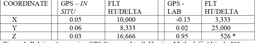
For the purpose of comparing geospatial accuracies produced by laboratory and by in situ calibrations, photogrammetric resections were computed producing spatial coordinates of the exposure stations. A Zeiss LMK 15/23 camera was used for this test. Comparisons were based on photography taken at typical large scale operational altitude of 500 meters above ground. For both cases of resection, one using the laboratory calibration and the other the calibration

produced from aerial photography (in situ), resected coordinate results were compared to the GPS positions, the independent standard of higher accuracy. Results of using a typical film based mapping camera, after comparing a number of sets of resected exposure stations, are presented in Table 1. These results are typical for film based mapping cameras compared over the last 20 years. Cause of such large elevation differences between laboratory and in situ calibrations may be lack of temperature corrections.

COORDINATE GPS – IN Figure 1. Relative Accuracies, GPS Compared to Calibration Methods@ Altitude 500 Meters [* Note: This proportional closure error exceeds the old, 3rd order survey closure error by a factor of 100)

Clearly, to improve geospatial accuracy, the concepts of calibration should follow an in situ approach and be in accord with Eisenhart.

POTENTIAL NGA APPLICATIONS

Viewing aerial analytical photogrammetry as having potential for providing high accuracy, geospatial coordinates by remote means; it then has application to NGA’s mission of providing accurate, reliable target locations on a timely basis. Use of unmanned aerial vehicles (UAV) for collection of intelligence is an important tool for such applications. It is the improvement in the current UAV intelligence collection technology, with emphasis on geospatial coordinates measurement accuracy that is the primary contribution made here to NGA’s research directions.

NGA will continue to be involved with the development of advanced geospatial data collection systems. Before calibration, these systems should demonstrate an adequate level of stability. Components of measurement systems may display high levels of stability; however, when operating as a system, stability in production of final measurements must also be demonstrated. To have a reasonable assurance of stability, the necessary number of measurements needs to be determined. After demonstration of adequate stability of a measurement system under

(20)

located at the USGS facility in Reston, Virginia. The crossroads represent the crossing banks of optical collimators. Collimators are set at seven and one half degree intervals radiating from the nadir. The range targets are set accordingly. This spatial geometry has been used for many years by USGS to accomplish calibration of film-based mapping cameras thus verifying the geometry of the range.

The new digital camera used to demonstrate the calibration procedures is the Zeiss RMK-D using the green head. The camera (green head) has a nominal focal length of 46.8 mm with a digital array size of 41.5 x 46.8 mm. It was flown at 3900 feet above the Buckeye Range, and located in a Piper Aztec aircraft operated by Midwestern Aerial Photography. Airborne control was provided by a L1/L2 GPS receiver. Base station control was provided by a CORS station located 5 miles north of the range. The calibration, after adjustment, provided an rmse of image observational residuals of 1.9 microns; a result indicating a quality of fit equal to those

experienced by laboratory calibrations.

CONCLUDING REMARKS

After reviewing the mission of NGA and current trends in geospatial data collection methods, some suggestions for further research and development can be made. Although the digital aerial metric camera has been the central data gathering device discussed here, other sensors such as multispectral sensors and LIDAR should be further analyzed for applications. These devices should be explored as more detailed mission requirements evolve.

In view of the NGA mission, the following research in photogrammetry should include:

assess metric stability as new systems develop

establish measurement system calibration procedures in accord with Eisenhart emphasize calibration concepts to UAV in field deployed applications

These recommendations are made with the objective of refining the metric, geospatial data collection systems of the NGA.

REFERENCES

American Society of Photogrammetry (1980) “Manual of Photogrammetry”, Fourth Edition, Falls Church, VA

Eisenhart, Churchill (1963) “Realistic Evaluation of the Precision and Accuracy of Instrument Calibration Systems” Journal of Research of the National Bureau Standards, Vol. 67C, No. 2, April/June 1963

(21)

Lapine, Lewis (1990) “Analytical Calibration of the Airborne Photogrammetric System Using A Priori Knowledge of the Exposure Station Obtained from Kinematic Global Positioning System Techniques” The Ohio State University, 1990

(22)

(23)

9

Remote Sensing: An Overview

Russell G. Congalton

Department of Natural Resources and the Environment University of New Hampshire

Forward

This paper presents a summary of current remote sensing technology. It begins with a historical review of the basics of this discipline. Current methodologies are then presented and discussed. The paper concludes with an examination of some future considerations. The material

summarized in this paper, as well as more detail on all of these topics, can be found in the classic remote sensing texts by Campbell (2007), Jensen (2005) and Lillesand, Kiefer, and Chipman (2008).

1. Introduction

Remote sensing can be defined as learning something about an object without touching it. As human beings, we remotely sense objects with a number of our senses including our eyes, our noses, and our ears. In this paper we will define remote sensing only as it applies to the use of our eyes (i.e., sensing electromagnetic energy) to learn about an object of interest. Remote sensing has both a scientific component that includes measurements and equations as well as a more artistic or qualitative component that is gained from experience.

The field of remote sensing can be divided into two general categories: analog remote sensing and digital remote sensing. Analog remote sensing uses film to record the electromagnetic energy. Digital remote sensing uses some type of sensor to convert the electromagnetic energy into numbers that can be recorded as bits and bytes on a computer and then displayed on a monitor.

2. Remote Sensing

2.1 Analog Remote Sensing

The first photograph was taken around 1826 and the first aerial photograph was taken from a balloon above Paris in 1858 (Jensen 2007). However, the real advantages of analog remote sensing were not evident until World War I and became even more important in World War II. The military advantages of collecting information remotely are obvious and the methods for using aerial photography were rapidly developed. By the end of World War II there was a large group of highly trained personnel capable of doing amazing things with aerial photographs.

The field of analog remote sensing can be divided into two general categories: photo

interpretation and photogrammetry. Photo interpretation is the qualitative or artistic component of analog remote sensing. Photogrammetry is the science, measurements, and the more

(24)

understanding of analog remote sensing. However, this paper will concentrate more on the photo interpretation component, especially how it relates to the development of digital remote sensing. It is interesting to note that photogrammetry can stand alone as its own discipline and has developed a large base of knowledge and applications. Early uses of digital remote sensing tended to not be very dependent on many of the concepts of photogrammetry. Recently,

however, with the increase in spatial resolution of many digital remote sensors, photogrammetry has again become a very relevant component of not only analog but also digital remote sensing.

Photo interpretation allows the analyst to deduce the significance of the objects that are of interest on the aerial photograph. In order to deduce the significance of a certain object, the interpreter uses the elements of photo interpretation. There are seven elements of photo

interpretation: (1) size, (2) shape, (3) site, (4) shadow, (5) pattern, (6) tone/color, and (7) texture. Each element by itself is helpful in deducing the significance of an object. Some objects can easily be interpreted from a single element. For example, the Pentagon building is readily recognized just based on its shape. However, the interpreter/analyst gains increased confidence in their interpretation if a greater number of elements point to the same answer. This concept is called “the confluence of evidence”. For example, if the object of interest looks like pointy-shaped trees and is in a regular pattern and the shapes are small and they cast a triangular shadow and the photo is from the New England states, then the analyst can be very certain in concluding that this area is a Christmas tree farm.

Photo interpretation is accomplished by training the interpreter to recognize the various elements for an object of interest. The training is done by viewing the aerial photos, usually

stereoscopically (i.e., in 3D), and then visiting the same areas on the ground. In this way, the interpreter begins to relate what an object looks like on the ground to what it looks like on the aerial photograph. The uses of the elements of photo interpretation aid the analyst in deducing the significance of the objects of interest.

(25)

11 Remote Sensing: An Overview

as magenta on a CIR photo. Vegetation that is stressed because of drought or pollution or insect infestation, etc. has lower NIR reflectance that is readily visible in a CIR photograph. This stress is then “visible” on the CIR photo before it is visible to the human eye.

2.2 Digital Remote Sensing

While analog remote sensing has a long history and tradition, the use of digital remote sensing is relatively new and was built on many of the concepts and skills used in analog remote sensing. Digital remote sensing effectively began with the launch of the first Landsat satellite in 1972. Landsat 1 (initially called the Earth Resources Technology Satellite – ERTS) had two sensors aboard it. The return beam vidicon (RBV) was a television camera-like system that was expected to be the more useful of the two sensors. The other sensor was an experimental sensor called the Multispectral Scanner (MSS). This device was an optical-mechanical system with an oscillating mirror that scanned perpendicular to the direction of flight. It sensed in four wavelengths

including the green, red, and two NIR portions of the electromagnetic spectrum. The RBV failed shortly after launch and the MSS became a tremendous success that set us on the path of digital remote sensing.

Since the launch of Landsat 1, there have been tremendous strides in the development of not only other multispectral scanner systems, but also hyperspectral and digital camera systems. However, regardless of the digital sensor there are a number of key factors to consider that are common to all. These factors include: (1) spectral resolution, (2) spatial resolution, (3) radiometric

resolution, (4) temporal resolution, and (5) extent.

2.2.1 Spectral Resolution

Spectral resolution is typically defined as the number of portions of the electromagnetic

spectrum that are sensed by the remote sensing device. These portions are referred to as “bands”. A second factor that is important in spectral resolution is the width of the bands. Traditionally, the band widths have been quite wide in multispectral imagery, often covering an entire color (e.g., the red or the blue portions) of the spectrum. If the remote sensing device captures only one band of imagery, it is called a panchromatic sensor and the resulting images will be black and white, regardless of the portion of the spectrum sensed. More recent hyperspectral imagery tends to have much narrower band widths with several to many bands within a single color of the spectrum.

Display of digital imagery for visual analysis has the same limitation as analog film (i.e., 3 primary colors). However, since digital imagery is displayed through a computer monitor, the additive primary colors (red, green, and blue) are used. Therefore, a computer display is called an RGB monitor. Again, a maximum of 3 bands of digital imagery can be displayed

(26)

image would appear just as our eyes would see it. However, many other composite images can be displayed. For example a Color Infrared Composite would display the green band through the blue component of the monitor, the red band through the green component, and the NIR band through the red component. This composite image looks just like a CIR aerial photograph. It is important to remember that only 3 bands can be displayed simultaneously and yet many different composite images are possible.

2.2.2 Spatial Resolution

Spatial resolution is defined by the pixel size of the imagery. A pixel or picture element is the smallest two-dimensional area sensed by the remote sensing device. An image is made up of a matrix of pixels. The digital remote sensing device records a spectral response for each

wavelength of electromagnetic energy or “band” for each pixel. This response is called the brightness value (BV) or the digital number (DN). The range of brightness values depends on the radiometric resolution. If a pixel is recorded for a homogeneous area then the spectral response for that pixel will be purely that type. However, if the pixel is recorded for an area that has a mixture of types, then the spectral response will be an average of all that the pixel encompasses. Depending on the size of the pixels, many pixels may be mixtures.

2.2.3 Radiometric Resolution

The numeric range of the brightness values that records the spectral response for a pixel is determined by the radiometric resolution of the digital remote sensing device. These data are recorded as numbers in a computer as bits and bytes. A bit is simply a binary value of either 0 or 1 and represents the most elemental method of how a computer works. If an image is recorded in a single bit then each pixel is either black or white. No gray levels are possible. Adding bits adds range. If the radiometric resolution is 2 bits, then 4 values are possible (2 raised to the second power = 4). The possible values would be 0, 1, 2, and 3. Early Landsat imagery has 6 bit resolution (2 raised to the sixth power = 64) with a range of values from 0 – 63. Most imagery today has a radiometric resolution of 8 bits or 1 byte (range from 0 – 255). Some of the more recent digital remote sensing devices have 11 or even 12 bits.

It is important to note the difference between radiometric resolution and dynamic range. The radiometric resolution defines the potential range of values a digital remote sensing device can record. Dynamic range is the actual values within the radiometric resolution for a particular image. Given that the sensor must be designed to be able to record the darkest and brightest object on the Earth, it is most likely that the dynamic range of any given image will be less than the radiometric resolution.

2.2.4 Temporal Resolution

(27)

and can acquire off-nadir imagery. This ability increases the revisit period (temporal resolution) of that sensor. However, there can be issues introduced in the image geometry and spectral response for images taken from too great an angle from vertical.

Temporal resolution often determines whether a particular remote sensing device can be used for a desired application. For example, using Landsat to monitor river flooding in the Mississippi River on a daily basis is not possible given that only one image of a given place is collected every 14 days.

2.2.5 Extent

Extent is the size of the area covered by a single scene (i.e., footprint). Typically, the larger the pixel size (spatial resolution), the larger the extent of the scene. Historically, satellite digital imagery covered large extents and had large to moderately large pixels. Recent, high spatial resolution digital sensors on both satellites and airplanes have much smaller extents.

3. Digital Image Analysis

Digital image analysis in digital remote sensing is analogous to photo interpretation in analog remote sensing. It is the process by which the selected imagery is converted/processed into information in the form of a thematic map. Digital image analysis is performed through a series of steps. These steps include: (1) image acquisition/selection, (2) pre-processing, (3)

classification, (4) post-processing, and (5) accuracy assessment.

3.1 Image Acquisition/Selection

Selection or acquisition of the appropriate remotely sensed imagery is foremost determined by the application or objective of the analysis and the budget. Once these factors are known, the analyst should answer the questions presented previously. These questions include: what spectral, spatial, radiometric, temporal resolution and extent are required to accomplish the objectives of the study within the given budget? Once the answers to these questions are known, then the analyst can obtain the necessary imagery either from an archive of existing imagery or request acquisition of a new image from the appropriate image source.

3.2 Pre-processing

Pre-processing is defined as any technique performed on the image prior to the classification. There are many possible pre-processing techniques. However, the two most common techniques are geometric registration and radiometric/atmospheric correction.

(28)

including: nearest neighbor, bilinear interpolation, and cubic convolution. The most commonly used approach has traditionally been cubic convolution. However, this technique uses an average computed from the nearest 9 pixels and has the effect of smoothing (or reducing the variance) in the imagery. Since this variance can represent real information in the imagery, smoothing the image is not always recommended. The nearest neighbor technique does not average the image, but rather uses the nearest pixel as the label for the registered pixel. However, linear features can be split between lines of imagery using the nearest neighbor technique. Bilinear interpolation also averages, but only uses the nearest 4 pixels. This approach represents a compromise between the other approaches. If the goal of the remote sensing analysis is to get the most information from the imagery, then the use of the nearest neighbor technique should be employed.

Radiometric/atmospheric correction is done to remove the effects of spectral noise, haze, striping and other atmospheric effects so that multiple dates or multiple scenes of imagery can be

analyzed together or so that the imagery can be compared to ground data. Historically, these corrections required collection of information about the atmospheric conditions during the time of the image acquisition. Algorithms/models used to correct for these effects relied on this ground information to accurately remove the atmospheric effects. More recently,

algorithms/models have been developed that use information gained from certain wavelengths in the imagery to provide the required knowledge to accomplish the correction. These methods are preferred given the difficulty of collecting the required ground data during image acquisition especially for imagery that has already been acquired.

3.3 Classification

Classification of digital data has historically been limited to spectral information (tone/color). While these methods attempted to build on the interpretation methods developed in analog remote sensing, the use of the other elements of photo interpretation beyond just color/tone has been problematic. The digital imagery is simply a collection of numbers that represent the spectral response for a given pixel for a given wavelength of electromagnetic energy (i.e., band of imagery). In other words, the numbers represent the “color” of the objects. Other elements of photo interpretation such as texture and pattern were originally not part of the digital

classification process.

In addition, digital image classification has traditionally been pixel-based. A pixel is an arbitrary sample of the ground and represents the average spectral response for all objects occurring within the pixel. If a pixel happens to fall on an area of a single land cover type (e.g., white pine), then the pixel is representative of the spectral response for white pine. However, if the pixel falls on an area that is a mixture of difference cover types (white pine, shingle roof, sidewalk, and grass), then the “mixel” is actually the areaweighted average of these various spectral responses.

(29)

3.3.1 Supervised vs. Unsupervised Classification

Supervised classification is a process that mimics photo interpretation. The analyst “trains” the computer to recognize informational types such as land cover or vegetation in a similar way that the photo interpreter trains themselves to do the same thing. However, the interpreter uses the elements of photo interpretation while the computer is limited to creating statistics (means, minimums, maximums, variances, and co-variances) from the digital spectral responses

(color/tone). The analyst is required to identify areas on the image of known informational type and create a training area (grouping of pixels) from which the computer creates a statistics file. Informational types that are rather homogeneous and distinct (e.g., water or sand) require only a few training areas. Complex, heterogeneous informational types (e.g., urban areas) require more training areas to adequately “train” the computer to identify these types. Supervised

classification works especially well when there are only a few (4-8) informational types that are distinctly different from each other.

Unsupervised classification uses a statistical clustering algorithm to group the pixels in the imagery into spectral clusters. These clusters are spectrally unique, but may not be

informationally unique. In other words, a single cluster may be a combination of a number of informational types (e.g., cluster 4 may be a combination of white pine and grass). The analyst decides how many clusters to use to group the imagery. Once the imagery has been grouped into the designated number of clusters, each cluster must be labeled with the corresponding

informational type (i.e., land cover or vegetation type). Labeling the clusters can be difficult and frustrating as many of the clusters will be a combination of two or more informational types. Also, many clusters will be small and intimate knowledge of the area may be necessary in order to label them. In most cases, this knowledge is lacking which is why the analyst is trying to generate a thematic map of the area using remote sensing. The major advantage of the

unsupervised classification technique is that all the spectral variation in the image is captured and used to group the imagery into clusters. The major disadvantage is that it is difficult to

informationally label all the clusters to produce the thematic map.

3.3.2 Combined Approaches

(30)

3.3.3 Advanced Approaches

Using supervised or unsupervised classification approaches only work moderately well. Even the combined approaches only improve our ability to create accurate thematic maps a little more than using each technique separately. Therefore, a large amount of effort has been devoted to developing advanced classification approaches to improve our ability to create accurate thematic maps from digital remotely sensed imagery.

While there are many advanced approaches, this paper will only mention three: Classification and Regression Tree (CART) analysis, Artificial Neural Networks (ANN), and Support Vector Machines (SVM). CART analysis is a non-parametric algorithm that uses a set of training data to develop a hierarchical decision tree. This decision tree is created using a binary partitioning algorithm that selects the best variable to split the data into separate categories at each level of the hierarchy. Once the final tree is generated, it can then be used to label all the unknown pixels in the image. CART analysis has become widely used in the last few years both for pixel-based and object-based image classification. The method is extremely robust and provides significantly better map accuracies than have been achieved using the more basic approaches.

The ANN approach to image classification has been applied for the last ten years or more. The approach also relies on a training data set like CART does. The power of the ANN is that it has the ability to “learn”. An ANN consists of a set of nodes (called neurons) that are connected by links and organized by layers. There are at least three layers: the input layer, the output layer, and the intermediate layer(s). The training data are used to build the model that creates the weighting used in the intermediate layer(s) to label the unknown pixels. While this approach seems to have great potential, the method is subject to over-fitting the data and unnecessary complexity.

Therefore, while much work is still being done on this technique, it has not experienced the same widespread adoption as CART.

SVM are derived from the field of statistical learning theory and have been used in the machine vision field for the last 10 years. More recently, these methods have been developed for use in creating thematic maps from remotely sensed imagery. SVM act by projecting the training data nonlinearly into feature space of a higher dimension than that of the input data. This projection is accomplished using a kernel function and results in a data set that now can be linearly separated. The ability to separate out the various informational classes in the imagery is a powerful

advantage. Like ANN, SVM is subject to over-fitting. However, a technique that is part of the analysis works to minimize this issue. The use of SVM is relatively new and offers great potential for creating thematic maps from digital imagery.

3.3.4 Object-based Approaches

By far the greatest advance in classifying digital remotely sensed data in this century has been the widespread development and adoption of object-based image analysis (OBIA). Traditionally, all classifications were performed on a pixel basis. Given that a pixel is an arbitrary delineation of an area of the ground, any selected pixel may or may not be representative of the

(31)

method increases the number of attributes such as polygon shape, texture, perimeter to area ratio and many others that can be used to more accurately classify that grouping of pixels.

Polygons are created from pixels in OBIA using a method called segmentation. There are a number of current image analysis software packages that provide the means of performing object-based image analysis. In all these algorithms, the analyst must select of series of parameters that dictate how the segments or polygons are generated. Depending on the parameters selected, it is possible to create large polygons that may incorporate very general vegetation/land cover types or very small polygons that may divide even a specific cover type into multiple polygons.

The power of the segmentation process is two-fold. First, the imagery is now divided into polygons that can, in many ways, mimic the polygons that may have been drawn by an analyst that was manually interpreting this same image. In this way, some of the additional elements of manual interpretation mentioned earlier in this paper become relevant for digital image analysis. Secondly, as previously mentioned, the creation of polygons results in a powerful addition of attributes about the polygons that can be used by the classification algorithm to label the polygons. Both these factors significantly add to our ability to create accurate thematic maps.

3.4 Post-processing

Post-processing can be defined as those techniques applied to the imagery after it has been through the classification process. In other words, any techniques applied to the thematic map. It has been said that one analyst’s pre-processing is another analyst’s postprocessing. It is true that many techniques that could be applied to the digital imagery as a pre-processing step may also be applied to the thematic map as a post-processing step. This statement is especially true of

geometric registration. While currently most geometric correction is performed on the original imagery, such was not always the case. Historically, to avoid resampling the imagery and potentially removing important variation (information), the thematic map was geometrically registered to the ground instead of the original imagery. In addition, there are a vast variety of filtering processes that can be performed on the original imagery to enhance or smooth the imagery that can also be used on the thematic map to accomplish similar purposes.

3.5 Accuracy Assessment

Accuracy assessment is a vital step in any digital remote sensing project. The methods

summarized here can be found in detail in Congalton and Green (2009). Historically, thematic maps generated from analog remotely sensed data through the use of photo interpretation were not assessed for accuracy. However, with the advent of digital remote sensing, quantitatively assessing the accuracy of thematic maps became a standard part of the mapping project.

(32)

Without assessing both positional and thematic accuracy it is impossible to determine the source of the errors.

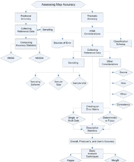
Conducting an accuracy assessment is not as simple as following a series of steps. Rather there are a number of important considerations that must be balanced between statistical validity and what is practically attainable. The outline in Figure 1 documents these considerations.

The basic processes for assessing positional accuracy and thematic accuracy are very similar. However, positional accuracy is simpler and involves fewer issues to consider than thematic accuracy. Positional accuracy provides an assessment of the difference in distance between a sample of locations on the map and those same locations on a reference data set. Sampling is performed because it is not possible to visit every location due to time, cost, and efficiency. There must be an adequate number of samples and these samples must be appropriately distributed across the map. A number of statistics are commonly computed including the root mean square error (RMSE) and the National Standard for Spatial Data Accuracy (NSSDA). The NSSDA is the national standard currently used in the US for positional accuracy. However, there is an error in the calculation of this measure that results in it being too conservative. This issue is currently being investigated for possible correction by a number of scientists and government agencies.

Assessing the thematic accuracy of a map uses the same basic process as assessing positional accuracy. However, a greater number of issues must be considered (see the more complicated flow chart in Figure 1). Thematic accuracy assessment involves a number of initial

considerations including taking into account the sources of error and the proper selection of a classification system. In addition, the collection of the reference data is more complicated including deciding the source of these data, how and when they will be collected, and insuring consistency in the collection process. Finally, sampling is a major component of the reference data collection. Sampling for thematic accuracy is much more complex than sampling for positional accuracy and requires selecting the appropriate sampling scheme along with the

sample size and sample unit. Sample size for thematic accuracy assessment is considerably larger than positional accuracy assessment and requires more careful planning to be as efficient as possible. While many thematic accuracy assessments have been conducted using the pixel as the sampling unit, this sampling unit is not appropriate as it fails to account for any positional error in the image and reference data. Therefore, a grouping of pixels or a polygon is the far better choice for a sampling unit.

Once the reference data are appropriately collected, the method used to compute thematic accuracy uses a technique called an error matrix. An error matrix is a cross tabulation or

(33)

(34)

It should be noted that Anderson et al. (1976) in a publication for the USGS stated that thematic maps generated from digital remotely sensed imagery should be at least 85 percent accurate. This value has been used as a guideline ever since. However, the overwhelmingly vast majority of thematic maps generated from remotely sensed data created from 1976 to the present have failed to meet this accuracy level.

4. Digital Image Types

4.1 MultiSpectral Imagery

The dominant digital image type for the last 40 years has been multispectral imagery from the launch of the first Landsat in 1972 through the launch of the latest GeoEye and DigitalGlobe sensors. Multispectral imagery contains multiple bands (more than 2 and less than 20) across a range of the electromagnetic spectrum. While there has been a marked increase in spatial

resolution, especially of commercial imagery, during these 40 years it should be noted that there is a solid place that remains for mid-resolution imagery. The importance of continuing imagery with a spatial resolution of 20-30 meters and with a good spectral resolution that includes the visible, near -, and middle infrared portions of the electromagnetic spectrum cannot be

understated. There is a special niche that this imagery fills that cannot be replaced by the higher spatial resolution imagery that costs significantly more to purchase. There will be increased uses of the higher spatial resolution data that continue to improve all the time, but this increase will not reduce the need for mid-resolution multispectral imagery.

4.2 Hyperspectral Imagery

Hyperspectral imagery is acquired using a sensor that collects many tens to even hundreds of bands of electromagnetic energy. This imagery is distinguished from multispectral imagery not only by the number of bands, but also by the width of each band. Multispectral imagery senses a limited number of rather broad wavelength ranges that are often not continuous along the

electromagnetic spectrum. Hyperspectral imagery, on the other hand, senses many very narrow wavelength ranges (e.g., 10 microns in width) continuously along the electromagnetic spectrum.

(35)

4.3 Digital Camera Imagery

Digital cameras are revolutionizing the collection of digital imagery from airborne platforms. These cameras sense electromagnetic energy using either a charged-coupled device (CCD) or a Complimentary Metal Oxide Semiconductor (CMOS) computer chip and record the spectral reflectance from an object with greater sensitivity than the old analog film cameras. While more expensive than analog film cameras, new digital camera systems, especially large format

systems, are rapidly replacing traditional analog systems. Large Federal Programs, such as the USDA National Agriculture Imagery Program (NAIP), are providing a tremendous source of digital imagery that the analyst can readily digitally analyze. Most digital camera imagery is collected as a natural color image (blue, green, and red) or as a color infrared image (green, red, and near infrared). Recently, more projects are acquiring all four wavelengths of imagery (blue, green, red, and near infrared). The spatial resolution of digital camera imagery is very high with 1 – 2 meter pixels being very common and some imagery having pixels as small as 15 cm.

4.4 Other Imagery

There are other sources of digital remotely sensed imagery that have not been presented in this paper. These sources include RADAR and LiDAR. Both these sources of imagery are important, but beyond the scope of this paper. RADAR imagery has been available for many years.

However, only recently has the multispectral component of RADAR imagery become available (collecting multiple bands of imagery simultaneously and not just multiple polarizations) that significantly improves the ability to create thematic maps from this imagery. LiDAR has

revolutionized the collection of elevation data and is an incredible source of information that can be used in creating thematic maps. In the last few years, these data have become commercially available and are being used as a vital part of many mapping projects.

5. Future Issues and Considerations

There are many issues and considerations related to the future of remote sensing. Four have been selected here for further discussion.

5.1 Software

(36)

5.2 Data Exploration Approach

The major reason that remotely sensed imagery can be used to create thematic maps is that there is a very strong correlation between what is sensed on the imagery and what is actually occurring in the same area on the ground. The key to making the most use of this correlation is through a process of data exploration. While there are many techniques that are part of most image analysis projects that provide insight into this correlation (e.g., spectral pattern analysis, bi-spectral plots, Principal Components Analysis, band ratios, vegetation indices, etc.), most analysts have not embraced a data exploration approach to accomplish their work. The statistics community has embraced this philosophy and has developed an entire branch of statistics for “data mining”. Incorporation of a similar philosophy of data exploration to investigate all aspects of the

correlation between the imagery and the ground could significantly improve our ability to create accurate thematic maps.

5.3 Landsat

Landsat is an invaluable source of remotely sensed imagery with a long history and an incredible archive. There is a tremendous need for the collection of imagery at this spatial and spectral resolution to continue well into the future. It is vital to our ability to look at global climate change, carbon sequestration, and other environmental issues that we have such imagery available. There is a need for a program to insure the future of Landsat and not simply a campaign each time a new Landsat is needed. Landsat imagery has become a public good and provides information that is not readily attainable anywhere else.

5.4 Remote Sensing and the General Public

Since the turn of the century, the general public has become increasingly aware of the use of remotely sensed imagery and geospatial technologies. Events such as the World Trade Center attack on September 11, 2001 and various natural disasters in New Orleans and elsewhere have made these technologies commonplace on the nightly news and the Internet. Applications such as Google Earth, Bing Maps, and others have given everyone the opportunity to quickly and easily use remotely sensed imagery anywhere in the world. This increased awareness and widespread understanding of these technologies is very positive. As more people become aware of the potential of these technologies more uses will be found for employing them for a myriad of applications.

6.0 Literature Cited

Anderson, J.R., E.E. Hardy, J.T. Roach, and R.E. Witner. 1976. A land use and land cover classification system for use with remote sensor data. USGS Professional Paper #964. 28 pp.

Campbell, J. 2007. Introduction to Remote Sensing. 4th edition. Guilford Press, New York. 626 p.

Chuvieco, E. and R. Congalton. 1988. Using cluster analysis to improve the selection of training statistics in classifying remotely sensed data. Photogrammetric Engineering and Remote

(37)

Congalton, R. and K. Green. 2009. Assessing the Accuracy of Remotely Sensed Data: Principles and Practices. 2nd Edition. CRC/Taylor & Francis, Boca Raton, FL 183p.

Congalton, R. 2010. How to Assess the Accuracy of Maps Generated from Remotely Sensed Data. IN: Manual of Geospatial Science and Technology, 2nd Edition. John Bossler. (Editor).

Taylor & Francis, Boca Raton, FL pp. 403-421.

Jensen, J. 2005. Introductory Digital Image Processing: A Remote Sensing Perspective. 3rd

edition. Pearson Prentice Hall. Upper Saddle River, NJ. 526p.

Jensen, J. 2007. Remote Sensing of Environment: An Earth Resource Perspective. 2ndedition.

Pearson Prentice Hall. Upper Saddle River, NJ. 592p.

Lillesand, T., R. Kiefer, and J. Chipman. 2008. Remote Sensing and Image Interpretation. 6th

(38)

(39)

25

Cartographic Research in the United States: Current Trends and

Future Directions

Robert McMaster Department of Geography

University of Minnesota

This white paper will focus on three basic areas of cartographic research: scale and

generalization, geographic visualization, and public participation mapping. It should be noted that the University Consortium for Geographic Information Science has developed and published a research agenda for GIS science, which consists of fourteen priorities, including (Usery and McMaster, 2004):

 Spatial Data Acquisition and Integration.  Cognition of Geographic Information  Scale

 Extensions to Geographic Representations

 Spatial Analysis and Modeling in a GIS Environment  Uncertainty in Geographic Data and GIS-Based Analysis  The Future of the Spatial Data Infrastructure

 Distributed and Mobile Computing

 GIS and Society: Interrelation, Integration, and Transformation  Geographic Visualization

 Ontological Foundations for Geographic Information Science  Remotely Acquired Data and Information in GIScience  Geospatial Data Mining and Knowledge Discovery

1.0SCALE AND GENERALIZATION

(Parts taken from Chapter 7, Thematic Cartography and Geographic Visualization, Vol. 3, Slocum, McMaster, Kessler, and Howard)

Geographic Scale

(40)

become the standard measure for map scale in cartography. The basic format of the RF is quite simple, where RF is expressed as a ratio of map units to earth units (with the map units standardized to 1). For example, an RF of 1:25,000 indicates that one unit on the map is equivalent to 25,000 units on the surface of the Earth. The elegance of the RF is that the measure is unitless—with our example the 1:25,000 could represent inches, feet, or meters. Of course, in the same way that 1

2 is a larger fraction than 14, 1:25,000 is a larger scale than 1:50,000.

Related to this concept, a scale of 1:25,000 depicts relatively little area but in much greater detail, whereas a scale of 1:250,000 depicts a larger area in less detail. Thus, it is the cartographic scale that determines the mapped space and level of geographic detail possible. At the extreme, architects work at very large scales, perhaps 1:100, where individual rooms and furniture can be depicted, whereas a standard globe might be constructed at a scale of 1:30,000,000, allowing for only the most basic of geographic detail to be provided. There are design issues that have to be considered when representing scales on maps, and a variety of methods for representing scale, including the RF, the verbal statement, and the graphical bar scale.

The term data resolution, which is related to scale, indicates the granularity of the data that is used in mapping. If mapping population characteristics of a city—an urban scale—the data can be acquired at a variety of resolutions, including census blocks, block groups, tracts, and even minor civil divisions (MCDs). Each level of resolution represents a different “grain” of the data. Likewise, when mapping biophysical data using remote sensing imagery, a variety of spatial resolutions are possible based on the sensor. Common grains are 79 meters (Landsat Multi-Spectral Scanner), 30 meters (Landsat Thematic Mapper), 20 meters (SPOT HRV multispectral), and 1 meter (Ikonos panchromatic). Low resolution refers to coarser grains (counties) and high resolution refers to finer grains (blocks). Cartographers must be careful to understand the relationship among geographic scale, cartographic scale, and data resolution, and how these influence the information content of the map.

Multiple-Scale Databases

Increasingly, cartographers and other geographic information scientists require the creation of multiscale/multiresolution databases from the same digital data set. This assumes that one can generate, from a master database, additional versions at a variety of scales. The need for such multiple-scale databases is a result of the requirements of the user. For instance, when mapping census data at the county level a user might wish to have significant detail in the boundaries. Alternatively, when using the same boundary files at the state level, less detail is needed. Because the generation of digital spatial data is extremely expensive and time-consuming, one master version of the database is often created and smaller scale versions are generated from this master scale. Further details are provided later.

(41)

27 Cartographic Research in the United States: Current Trends and Future Directions

The conceptual elements of generalization include reducing complexity, maintaining spatial accuracy, maintaining attribute accuracy, maintaining aesthetic quality, maintaining a logical hierarchy, and consistently applying the rules of generalization. Reducing complexity is perhaps the most significant goal of generalization. The question for the cartographer is relatively straightforward: How does one take a map at a scale of, perhaps, 1:24,000 and reduce it to 1:100,000? More important, the question is how the cartographer reduces the information content so that it is appropriate for the scale. Obviously, the complexity of detail that is provided at a scale of 1:24,000 cannot be represented at 1:100,000; some features must be eliminated and some detail must be modified. For centuries, through considerable experience, cartographers developed a sense of what constituted appropriate information content. The set of decisions required to generalize cartographic features based on their inherent complexity is difficult if not impossible to quantify, although as described next, several attempts have been made over the past two decades.

Clearly, there is a direct and strong relationship among scale, information content, and generalization. John Hudson explained the effect of scale by indicating what might be depicted on a map 5 by 7 inches:

• A house at a scale of 1:100 • A city block at a scale of 1:1,000

• An urban neighborhood at a scale of 1:10,000 • A small city at a scale of 1:100,000

• A large metropolitan area at a scale of 1:1,000,000 • Several states at a scale of 1:10,000,000

• Most of a hemisphere at a scale of 1:100,000,000

• The entire world with plenty of room to spare at a scale of 1:1,000,000,000

He explained that these examples, which range from largest ( :1102) to smallest ( :1109), span eight orders of magnitude and a logical geographical spectrum of scales. Geographers work at a variety of scales, from the very large—the neighborhood—to the very small—the world. Generalization is a key activity in changing the information content so that it is appropriate for these different scales. However, a rough guideline that cartographers use is that scale change should not exceed 10. Thus if you have a scale of 1:25,000, it should only be used for

generalization up to 1:250,000. Beyond 1:250,000, the original data are “stretched” beyond their original fitness for use.

(42)

When Generalization Is Required

In a digital cartographic environment, it is necessary to identify those specific conditions when generalization will be required. Although many such conditions can be identified, four of the fundamental ones include:

1. Congestion 2. Coalescence 3. Conflict 4. Complication

As explained by McMaster and Shea, congestion refers to the problem when, under scale reduction, too many objects are compressed into too small a space, resulting in overcrowding due to high feature density. Significant congestion results in decreased communication of the mapped message, for instance, when too many buildings are in close proximity. Coalescence refers to the condition in which features graphically collide due to scale change. In these situations, features actually touch. This condition thus requires the implementation of the displacement operation, as discussed shortly. Conflict results when, due to generalization, an inconsistency between or among features occurs. For instance, if generalization of a coastline eliminates a bay with a city located on it, either the city or the coastline must be moved to ensure that the urban area remains on the coast. Such spatial conflicts are difficult to both detect and correct. The condition of complication is dependent on the specific conditions that exist in a defined space. An example is a digital line that changes in complexity from one part to the next, such as a coastline that progresses from very smooth to very crenulated, like Maine’s coastline.

Despite the fact that many problems in generalization require the development and implementation of mathematical, statistical, or geometric measures, little work on generalization measurement has been reported. Two basic types of measures can be identified: procedural and quality assessment. Procedural measures are those needed to invoke and control the process of generalization. Such measures might include those to: (1) select a simplification algorithm, given a certain feature class; (2) modify a tolerance value along a feature as the complexity changes; (3) assess the density of a set of polygons being considered for agglomeration; (4) determine whether a feature should undergo a type change (e.g., area to point) due to scale modification; and (5) compute the curvature of a line segment to invoke a smoothing operation. Quality assessment measures evaluate both individual operations, such as the effect of simplification, and the overall quality of the generalization (e.g., poor, average, excellent).

A Framework for the Fundamental Operations

NGA Workshop Whitepapers

National Research Council

Workshop on New Research Directions for the

National Geospatial-Intelligence Agency

White Papers

Workshop on New Research Directions for the

National Geospatial-Intelligence Agency

White Papers

Table of Contents

Calibration of the Aerial Photogrammetric System

Remote Sensing: An Overview

Cartographic Research in the United States: Current Trends and

Future Directions