www.elsevier.com / locate / livprodsci
Evaluation of models for somatic cell score lactation patterns in
Holsteins
*
Sandra L. Rodriguez-Zas , Daniel Gianola, George E. Shook
Department of Dairy Science, University of Wisconsin, Madison, WI 53706, USA
Received 2 June 1999; received in revised form 16 February 2000; accepted 16 March 2000
Abstract
Milk somatic cell score (SCS) typically reaches a minimum early in lactation and then rises. Nonlinear mixed effects models were used to describe this trajectory while accounting for between and within-cow variation. A total of 2387 SCS records from 217 Holsteins were analyzed. Four nonlinear and two linear functions were studied. Approximate maximum likelihood estimates indicated that cows free of intramammary infection had sharper SCS decreases after calving, and lower overall levels. Lactations starting between October and December had the highest fall of SCS levels at the beginning of lactation, and the smallest increases thereafter. In general, there was significant variation between cows’ individual trajectories. For some parameters and models, however, this variation was small. A four-parameter model suggested by Morant and Gnanasakthy was supported better by the data than the other five functional forms. 2000 Elsevier Science B.V. All rights reserved.
Keywords: Longitudinal data; Maximum likelihood; Nonlinear mixed effects models; Mastitis
1. Introduction indicator of udder health status for management and
selection purposes.
Mastitis is an udder health disorder that causes After the beginning of lactation, SCS decreases to
substantial economic losses to the dairy industry a minimum at around 60 days post-calving and
(Shook, 1989). This inflammation of the mammary increases thereafter (Wiggans and Shook, 1987).
gland, usually in response to invasive agents, can be Variation in the shape and level of the SCS pattern is
characterized by an increase in the somatic cell count related to lactation number (Wiggans and Shook,
(SCC) in milk. This trait or a logarithmic transform, 1987), to udder infection status (Sheldrake et al.,
called somatic cell score (SCS), is used as an 1983) and to individual cows. Heritability estimates
of test-day SCS range between 0.07 and 0.44 (Ali and Shook, 1980; Kennedy et al., 1982; Emanuelson and Philipsson, 1984; Gadini et al., 1996). Monardes
*Corresponding author. Department of Animal Sciences,
Uni-and Hayes (1985) reported repeatability estimates of
versity of Illinois at Urbana-Champaign, Urbana, IL 61801, USA.
test-day SCS of 0.36–0.42 across parities, and
Tel.: 11-217-333-8810; fax:11-217-333-8286.
E-mail address: [email protected] (S.L. Rodriguez-Zas). repeatability within lactations ranged from 0.47 to
0.59 (Emanuelson and Persson, 1984). These results recorded between July 1982 and June 1989. The herd
suggest the need to consider both the variation within was maintained free of Streptococcus agalactiae, and
and between cows for an adequate modeling of SCS less than 1% of the quarters were infected with
trends. Further, an important fraction of the variation Staphylococcus aureus at any one time (Todhunter et
seems to be related to genetic factors. al., 1991). The bacteriological status was assessed by
Lactation average SCS measures are used current- 0.01 ml of milk streaked onto the surface of a 0.25
ly in some national genetic evaluation schemes, the plate of Trypticase soy agar containing 5% whole
objective being to lower the prevalence of mastitis bovine blood and esculin (Smith et al., 1985).
Forty-by indirect selection for SCC. This approach does five percent of the test-day observations were
nega-not use all the information and masks short-term tive for IMI. The two most common pathogens were
variation in SCS (Shook and Schutz, 1994; Emanuel- Staphylococcus spp. (excluding Staphylococcus
au-son, 1997). Test-day somatic cell records are taken reus) and Corynebacterium spp. (31 and 15% of the
on the same cow at various times, providing longi- observations, respectively). Approximately 10% of
tudinal information that can be related more mean- the observations were associated with clinical
mas-ingfully to episodes of infection. A statistical model titis symptoms. A description of the herd
man-for longitudinal data may provide more accurate agement-health practices is in Smith et al. (1985)
estimates of the influence of risk factors than lacta- and Todhunter et al. (1991). Milk samples were
tion average models. This additional information taken on each cow at 14 and 30 days in lactation,
should be beneficial in the study of a trait with and every 30 days thereafter until the end of lactation
seemingly low heritability, such as SCS. or 300 days in milk, whichever occurred first. Each
A reasonable model for describing SCS variation milk sample was tested for presence of pathogens
during lactation must consider the ‘typical’ lactation and SCC was assessed electronically using a Coulter
pattern and allow for differences associated with Counter. Here: SCS531log (SCC / 100) where2
explanatory variables (e.g. age of cow) and with the SCC is in cells /ml.
individual cows themselves. Nonlinear mathematical A binary variable describing intramammary
in-functions are natural candidates for describing SCS fection status (IMI) was created for each
cow-lacta-lactation patterns, and their parameters can be tion. A single positive pathogen isolation (e.g.
bac-modeled to account for known sources of variation. teria, yeast) during lactation was enough to code IMI
Estimates of these parameters can be used for as ‘one’; otherwise, it was coded as zero. Most
management and breeding purposes to the extent that cow-lactations that were free of infection early in
at least some of the variation detected is heritable. lactation (91% of all cow-lactations) remained so
The main objective of this study was to explore until the end of lactation. Similarly, most cows that
the feasibility of nonlinear mixed effects models to were culture-positive after calving remained positive
describe the SCS lactation curves. Another objective in subsequent test-days (84%). Roughly the same
was to compare the fit of four nonlinear models and number of cows was positive for IMI at every test
two linear models when applied to SCS lactation day with values ranging between 107 cows at 14
records in Holstein cows. An approximate maximum days and 128 cows at 300 days. The majority of the
likelihood analysis was used for these purposes. cows positive for IMI at one test-day were positive
in subsequent test-days. Eight percent of all the lactations had one, two or three infection episodes.
2. Materials and methods Obviously, a single measure of IMI status does not
capture the dynamics of infection in the course of
2.1. Data lactation and does not differentiate between a cow
positive for pathogen isolation at 30 days, and one
The Ohio Agricultural Research and Development being positive at the last 3 test-days. This way of
Center (Wooster) provided the SCC data used. After coding IMI is time independent however, and can be
edits, the data consisted of 2387 test-day observa- permitted to be included as a covariate for the
evaluated as modulator of the SCS trends. Better indicated that the normality assumption was adequate
forms of modelling SCS pattern may include test-day (Rodriguez-Zas, 1998). The cow effects represent a
IMI status. Alternative ways of accounting for the combination of genetic and permanent environmental
dynamics of IMI infection during lactation are effects, and these were assumed to be independent
considered in Section 4. from the residuals. Although cow effects were
The calvings in 1983, 1984 and 1985 were assumed to be independent, this assumption can be
grouped in period 1; calvings in 1986 and 1987 were relaxed; the independence assumption was used in
in period 2, and period 3 included 1988 and 1989 view of the sparse structure of the genetic
relation-calvings. Months of calving were grouped into four ship matrix between cows. The matrix S is a
seasons: season 1 included calvings from January 1 positive-definite matrix containing variances and
2
through March 31, and so on. Lactations were coded covariances of cow effects on parameters ands is
as first, second or third. To be included in the data the residual variance. Hence, conditionally on the
set, cows in a given lactation needed to have records cow effects, the observations had a Gaussian
dis-in the preceddis-ing ones. However, there were animals tribution with mean f (iui) and unknown,
homos-2
with first lactations without second lactations, etc. cedastic, variance s . The assumption of constant
residual variance was made following Shook (1982). A preliminary time series analysis gave no indication 2.2. Statistical procedures
of violation of the assumption of lack of correlation between residuals within cows.
The nonlinear mixed effects models used here can be represented with two equations:
2.3. Approximate maximum likelihood estimation
yi5f (iui)1ei (1)
2
The unknown parameters (b, S, s ) were
esti-u 5i Xib 1Z b .i i (2) mated by maximizing an approximation to the
likelihood function. The joint density of all
observa-Eq. (1) describes how the longitudinal data are tions, conditionally on the random effects is:
generated given a nonlinear function f (iui). Here, yi
M
is an ni31 vector of test-day SCS of the ith cow 2 2
p(yub, b,s )5
P
p(yiub, b ,i s )9 9 9
(y5[y , y , . . . , y ]1 2 M 9) and M is the number of cows; i51
ui is an r31 vector of parameters peculiar to the ith
with cow; f (iui) is an ni31 vector of expected values
(given ui) of scores of cow i and e is an ni i31 2 2
yiub, b ,i s |N[f (i b, b ),i s I ].ni (3)
vector of residuals. The second equation expresses
how the parametersuivary according to explanatory
The marginal density of y results from integrating variables b (fixed) and b (random). In (2) X is ani i
over R , the sampling space of the random effects:b
r3p incidence matrix relating fixed effects ( p5
number of uniquely estimable fixed effects) toui; b
2 2
is a p31 vector of fixed effects affectingui; Z is ani p(yub,S,s )5
E
p(yub, b,S,s ) p(buS)≠b (4)incidence matrix of appropriate order relating the Rb
random effects b (ri 31) toui. Note that each cow
where p(bu S) is the density of the sampling
has an effect on each of theuiparameters so (1) and
distribution of the random effects. These effects (2) embed a multivariate structure within a
uni-were assumed to be independent, thus p(bu S)5
variate longitudinal model.
M
Random variables in (1) and (2) are the cow
P
i51p(biu S). The required integration is complex2
effects bi|NIID (0, S) and ei|N(0,s I ), whereni because of the nonlinear relation between the
ob-NIID denotes normal, independent and identically servations and the random effects. The residual or
distributed. An analysis of these models in a restricted likelihood obtained after integration of b
2 2sNM / 2d 21 / 2 21 / 2 ˆ ˆ ˆ ˆ ˆ
,
s
S,s uyd
5s2pd u uR uI^Su y¯f(b, b )1X(b 2 b)1Z(b2b )1e (8)i
1 21 or equivalently
]
distribution of the pseudo-data vector is:
M 2
where N5oi51n , Ri 5Is in the present study and ˆ
y*|N(Xb, V ) (10)
f(b, b)5hf (i b, b )i j is the conditional expectation
(givenb and b) of the observations. The integration ˆ ˆ 2
where V5Z (I^S) Z9 1Is (Wolfinger and Lin,
in Eq. (5) cannot be done analytically (due to
1997). Then the restricted or residual log-likelihood nonlinearity), a Laplacian approximation proposed
(based on y*) is approximately: by Wolfinger (1993) and Wolfinger and Lin (1997)
2 1 1
was used. At a given value of S and s , the ˜ 2 ˆ 21ˆ
] ]
,
s
S,s uy*d
5constant2 loguX9V Xu2 log Vu u2 2
Laplacian approach consists in approximating the
integral in (5) with a second-order Taylor series ]1
s
ˆd
21s
ˆd
2 y*2Xb 9V y*2Xb. (11) ˆ
expansion centered at the mode of the maximizers b 2
ˆ
and b of the ‘penalized log likelihood’:
This has the same form as the log-restricted
21
likelihood for a linear mixed effects model, so any
2(1 / 2)h[y2f(b, b)]9R [y2f(b, b)]
standard REML algorithm can be applied to obtain
21
1b9(I^S) bj. (6) 2
new values of S and s . The process iterates
between the maximum penalized likelihood step (7)
ˆ ˆ
Letting X5 ≠fsb, b /d ≠b9 and Z5 ≠fsb, b /d ≠b9 and the REML search (11). Whenever (1) is linear in
and using Fisher’s method of scoring to locate the the parameters, (7) leads to BLUP and (11) is
mode leads to the iterative system: exactly the restricted log-likelihood. The standard
errors of the estimates of the variance components
ftg t11
21 21 f g
ˆ ˆ ˆ ˆ
X9R X X9R Z b
can be computed from the inverse of the estimated
F
ˆ 21ˆ ˆ 21ˆ 21G F G
Z9R X Z R Z1V b information matrix. To assess whether a random
ftg
21
ˆ effect should be removed from the model a
likeli-X9R y*
5
F
21G
(7) hood ratio test was used. Computations were carriedˆ
Z9R y*
out with SAS 6.11 (SAS Institute Inc., 1996).
21
Here, t denotes iteration number, V 5
21 ˆ ˆ ˆ ˆ
2.4. Models describing SCS trajectory
I^S and y*5y2f(b, b )1Xb 1Z b is a
pseu-ˆ pseu-ˆ
do-data vector. The matrices X, Z and the vector y*
The nonlinear functions represented by (1) used to need to be evaluated at each iteration, starting from
describe SCS lactation patterns were: an arbitrary b0 and b .0
2
Given S and s , the inverse of the coefficient
ˆ ˆ 1. Wood’s (1967) equation (W):
matrix of (7) evaluated at b and b gives,
approxi-mately, the variance-covariance matrix of the esti- b
yij5a (t ) exp(ij 2dt )ij 1eij (12) mates of fixed effects and of the prediction errors of
the random effects b. Maximizing the penalized log where yij and tij are the SCS and test-day,
likelihood (6) gives the same estimating equations respectively, of observation j taken on cow i. The
obtained by Gianola and Kachman (1983) and parameters are: a, associated to SCS level at the
Kachman (1985) in a Bayesian setting with flat beginning of lactation; b, a declining slope
param-priors for b and known variance components. With eter, and d an increasing slope parameter.
the new values of b and b model (1) can be 2. An inverse quadratic (IQ) model studied by
2
yij5[t /(aij 1btij1dt )]ij 1e .ij (13) of lactation and a with the decrease after calving.2
The constant 20.05 is related to the time at
Parameter a describes the rate of decrease after minimum SCS, expected to occur at about 50
calving, d is the increase on SCS level at the end days post-partum. Linear mixed effects model
of lactation and b is a scale parameter. methodology was used to analyze AS and WI
3. Mitscherlich’s model with an exponential term models, because these are linear in the
parame-(Rook et al., 1993), or ME, can be expressed as: ters. In all the models considered (linear and
nonlinear), the parameters at the second stage yij5[12a exp(bt )] exp(ij 2dt )ij 1e .ij (14)
have a varying degree of collinearity. Parameter a describes the curve’s scale, b gives
the rate of decrease at early stages of lactation 2.5. Models for describing parameter variation
and d is associated to the rate of increase in SCS
observed after a minimum has been reached. Parameters for each of the six models were
4. Morant and Gnanasakthy (1989), or MG, is the described as a linear combination of fixed effects and
four-parameter model: of random effects peculiar to each cow. The full
model had the form: acterizes the expected SCS at day 150 of lactation
and b represents the relative rate at which SCS
whereuijklmis a parameter (of any of the models); m
changes at 150 days of lactation (% per day).
is a constant; IMI is a fixed effect of infection statusi Parameter d measures the extent to which the rate
i (i50, 1) during lactation; P is a fixed effect ofj of increase in SCS changes during lactation and f
period of calving j ( j51, 2, 3); S is a fixed effectk is related to the rate of decrease in SCS early in
of season of calving k (k51, 2, 3, 4); L is a fixedl lactation.
effect of lactation number l (l51, 2, 3); bijklm is a 5. Ali and Schaeffer (1987) proposed the
five-pa-regression of the parameter on age at calving for the rameter model (AS):
current lactation and cow; Aijklm is the age at calving
2 of cow m with infection status i, calving in period j
yij5b01b (t / 300)1 ij 1b (t / 300)2 ij
and season k and with lactation number l; bm is a
2
1b log(300 /t )3 ij 1b [log (300 /t )]4 ij 1e .ij random effect peculiar to the appropriate parameter of cow m. Two-factor interactions were not signifi-(16)
cant. For each model, effects not different from zero
The b parameters do not have a mechanistic (P,0.01), based on likelihood ratios and t-tests were
interpretation although the second and third terms removed from the model. A strategy based on the
are related to the rate of increase of SCS at mid eigenvalues of S suggested by Pinheiro and Bates
and late lactation, and the fourth and fifth parame- (1997) for identifying random effects to be included
ters describe the fall at the beginning of the in the model was used. Results were corroborated
lactation. using significance tests for dispersion components
6. Wilmink’s (1987) model (WI) was included in (Self and Liang, 1987). In theory, the assumption of
the study. The three-parameter model was: unrelatedness between cows and of independence
between lactations of the same cow leads to under-yij5a01a t1 ij1a exp(2 20.05t )ij 1e .ij (17)
estimation of the asymptotic standard errors of the
Actually, this is a four-parameter model, the maximum likelihood estimates. Hence, final models
fourth one being set equal to 20.05 to improve may have more parameters than actually needed.
numerical behavior. Parameter a0 is associated However, the relationship matrix was very sparse
with a baseline level of SCS, a with the increase1 (88% of the off-diagonal elements of the relationship
serious problem. Comparisons between non-nested high levels of SCS, causing the average to be higher
models relied on Akaike’s Information Criteria (AIC; than the values usually associated to minor
patho-Akaike, 1974) and on Schwarz’s Bayesian Criterion gens. As shown in Table 1, SCS decreased to a nadir
(BIC; Schwarz, 1978), both of which adjust likeli- at about 60 DIM and then increased, although not in
hood ratio tests by the number of parameters in the a monotonic fashion, without regaining the initial
model. Also, the residual variance was used to level. The standard deviation followed an inverse
compare models. pattern. All parameter estimates presented
sub-sequently are from the reduced models, as mentioned earlier. In all models, lactation number was not a
3. Results significant source of variation for any of the
parame-ters.
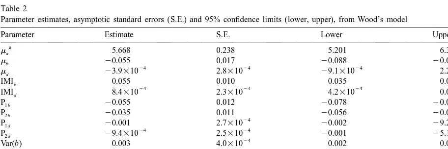
Mean 305-day, mature equivalent milk yield was Estimates from Wood’s model (Table 2) indicate
about 7600 kg. Average SCC and standard deviation that intramammary infection status affects the two
was 671,000 and 897,000 cells / ml, respectively. A shape parameters (b and d ). The a scale parameter
few cows, with clinical mastitis symptoms, have very was higher in infected animals, but the difference
was not significant. This is sensible because the IMI variable pertains to status during and not at the onset
Table 1
Average somatic cell score and standard deviation (S.D.) by of lactation. Animals that had positive pathogen
test-day isolations during lactation had a less sharp fall in
Days in milk Mean S.D. SCS at the beginning of lactation (positive parameter b estimate when IMI51) than cows free of infection
14 5.425 1.418
throughout lactation. However, infected cows had
30 4.910 1.519
60 4.875 1.616 steeper rates of increase after nadir (positive
parame-90 5.096 1.463 ter d estimate when IMI51) than non-infected cows.
120 5.105 1.295
The period of calving affected the shape parameters
150 5.132 1.386
significantly: cows calving in period 3 (last 3 years
180 5.264 1.331
of the trial) tended to have larger b and d values than
210 5.017 1.274
240 5.171 1.296 those calving at periods 1 or 2. The between-cow
270 5.163 1.357 variation was significant for parameters b and d. The
300 5.038 1.374
variance components cannot be expressed in terms of
Table 2
Parameter estimates, asymptotic standard errors (S.E.) and 95% confidence limits (lower, upper), from Wood’s model
Parameter Estimate S.E. Lower Upper
a
ma 5.668 0.238 5.201 6.314
mb 20.055 0.017 20.088 20.023
24 24 24 24
md 23.9310 2.8310 29.1310 2.2310
IMIb 0.055 0.010 0.035 0.075
24 24 24
Var(b) 0.003 4.0310 0.002 0.004
26 26 27 26
Var(d ) 1.2310 3.8310 7.7310 3.1310
25 26 25 25
Cov(b, d ) 4.7310 8.6310 2.9310 7.7310
Var(e) 1.181 0.038 1.110 1.258
a
mi, intercept for parameter i; IMI , effect of presence of intramammary infection; P , effect of the k period of calving as a deviation fromi ki
fractional contribution to the total variance because such cows had higher levels of somatic cells when a
of the nonlinearity. The residual variance is in the minimum had been reached. All components of
SCS scale (Eq. (1)), whereas the components are dispersion were significant and the random effects
expressed at the level of the parameters (Eq. (2)). had a strong intercorrelation that could have
conse-The correlation between random effects affecting quences in selection for specific features of the SCS
parameters b and d was about 0.78, suggesting that pattern.
cows with rapid decline of SCS early in lactation With the ME model (Table 4), only IMI status and
tend to regain levels slowly after nadir. cow were significant sources of variation. Infected
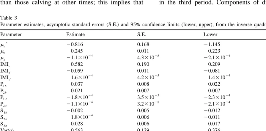
The presence of intramammary infection affected cows had lower values of parameter a, which means
all three parameters of the IQ model (Table 3). The a higher baseline SCS level. The four parameters
infected cows had a slower rate of decrease of SCS were strongly intercorrelated, especially b and d,
in early lactation (larger parameter a), and a some- which had an almost perfect correlation. This
sug-what higher rate of increase in late lactation (positive gests potential computational problems (at least with
estimates of parameter d ) than healthy cows. The the present data structure), thus estimates should be
SCS curve tended to be ‘flatter’ in the presence of interpreted with caution.
infection (positive estimates of parameter d and The estimates obtained from the MG model are in
negative estimates of parameter b describing the fall Table 5. Presence of intramammary infection
in-and follow up increase in SCS levels, respectively), creased the level of somatic cell score (parameter a),
in agreement with results from Wood’s model. decreased the rate of increase of SCS at 150 days
Period affected variation in b and d parameters after calving (parameter b) and reduced the rate of
significantly. Season of calving affected only the fall of somatic cell levels immediately after calving
scale parameter b. Cows calving in seasons 2 and 3 (parameter f ). Parameter b was higher in cows that
(April–September) had larger b parameter estimates calved in the first period and lower for cows calving
than those calving at other times; this implies that in the third period. Components of dispersion and
Table 3
Parameter estimates, asymptotic standard errors (S.E.) and 95% confidence limits (lower, upper), from the inverse quadratic model
Parameter Estimate S.E. Lower Upper
a
ma 20.816 0.168 21.145 20.487
mb 0.245 0.011 0.223 0.268
24 25 24 26
md 21.1310 4.3310 22.1310 21.3310
IMIa 0.582 0.190 0.209 0.955
IMIb 20.059 0.011 20.081 20.037
24 25 24 24
IMId 1.6310 4.2310 1.4310 2.1310
P1b 0.037 0.008 0.022 0.052
P2b 0.021 0.007 0.007 0.034
24 25 24 24
S3b 0.028 0.006 0.017 0.039
Var(a) 0.563 0.129 0.376 0.933
24
Var(b) 0.003 4.7310 0.002 0.004
28 28 28 28
Var(e) 1.102 0.037 1.031 1.178
a
mi, intercept for parameter i; IMI , effect of presence of intramammary infection; P , effect of the k period of calving as a deviation fromi ki
the third one; S , effect of the k season of calving as a deviation from the fourth one; Var(i ), variance for parameter i; Cov(i, j ), covarianceki
Table 4
Parameter estimates, asymptotic standard errors (S.E.) and 95% confidence limits (lower, upper), from the Mitscherlich-exponential model
Parameter Estimate S.E. Lower Upper
a
Var(a) 1.314 0.219 0.972 1.877
24 24 24 24
Var(e) 1.095 0.037 1.025 1.172
a
mi, intercept for parameter i; IMI , effect of presence of intramammary infection; Var(i ), variance for parameter i; Cov(i, j ), covariancei
between parameters i and j; Var(e), residual variance.
Table 5 (parameter a) would be expected to have a more
Parameter estimates, asymptotic standard errors (S.E.) and 95% variable rate of increase of SCS in the middle of confidence limits (lower, upper), from the Morant and
Gnanasak-lactation.
thy’s model
Fixed factors were not a significant source of
Parameter Estimate S.E. Lower Upper
variation in any of the linear regression parameters
a
ma 4.292 0.120 4.057 4.526 of Ali and Schaeffer’s model, but there was
signifi-mb 0.060 0.022 0.016 0.104 cant variation and covariation between cows. In 24
md 20.020 0.011 20.040 9.1310
Wilmink’s model, presence of intramammary
in-mf 4.737 0.814 3.139 6.334
fection was associated with higher levels of SCS
IMIa 0.853 0.137 0.584 1.121
IMIb 20.074 0.021 20.115 20.034 during lactation, in agreement with W, IQ and MG
IMIf 22.791 0.860 24.478 21.105 models. Cows calving on the first and second periods P1b 0.096 0.019 0.060 0.132 had lower a values than those calving in the third
P2b 0.062 0.017 0.029 0.096
period, and higher increases in SCS levels in mid
Var(a) 0.742 0.093 0.589 0.964
and late lactation. There was significant variation
Var(b) 0.006 0.001 0.004 0.009
Var(d ) 0.008 0.001 0.005 0.011 between cows for parameters of this model.
Cov(a, b) 0.008 0.007 20.005 0.022 Numerical values of end-points used for compar-Cov(a, d ) 20.049 0.010 20.069 20.030 ing models are in Table 6. The Ali and Schaeffer’s
24 24
Cov(b, d ) 20.001 8.6310 20.003 5.2310 Var(e) 1.043 0.035 0.977 1.116
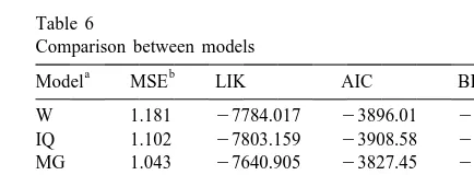
Table 6 a
mi, intercept for parameter i; IMI , effect of presence ofi Comparison between models
intramammary infection; P , effect of the k period of calving as aki
a b
Model MSE LIK AIC BIC
deviation from the third one; Var(i ), variance of parameter i;
Cov(i, j ), covariance between parameters i and j; Var(e), residual W 1.181 27784.017 23896.01 23907.56
variance. IQ 1.102 27803.159 23908.58 23928.78
MG 1.043 27640.905 23827.45 23847.66 ME 1.095 27720.616 23867.31 23887.52
co-dispersion for parameters a, b and d were
signifi-AS 0.950 27644.072 23838.04 23884.24
cant indicating differences between cows in the
WI 1.098 27707.943 23860.97 23881.18
shape and scale of SCS lactation curves. In spite of
a
W, Wood’s; IQ, inverse quadratic; MG, Morant and
Gnanasak-being a four-parameter model, the correlation
struc-thy’s; ME, Mitscherlich-exponential; AS, Ali and Schaeffer’s; WI,
ture between random effects was weaker than for the
Wilmink’s model.
other models. Only random effects affecting parame- b
MSE, residual variance; LIK, 23maximized restricted
log-ters a and d had a sizable (20.64) correlation, likelihood; AIC, Akaike’s information criterion; BIC, Schwarz’s
(AS) model had the lowest residual variance, but the the second most common quarter isolation in the
largest number of parameters; the ME model was Hogan et al. (1989) study, but the number of
second and the one with the poorest fit (in the MSE infected quarters ranged between 1% (calving) and
sense), was Wood’s. The MG model had the largest 8.8% (drying off), the latter being close to the
maximized restricted likelihood, followed by AS. incidence found in this data set. An improvement in
Based on Akaike’s and Schwarz’s criteria, the MG the management-health conditions during the study
model was better, followed by AS or WI, depending may be reflected by the lower rate of increase of SCS
on the criterion considered. The residuals plots did found in the third period of calving (MG model) and
not exhibit any patterns, suggesting that the model by the lower predicted values for this period (W
assumptions were suitable. model). The relatively warm and humid conditions
during peak lactation experienced by cows calving between July and September may have facilitated
4. Discussion contamination and prevalence of pathogens. This
would explain the higher values of parameter b for
The overall trend of SCS during lactation is cows calving in season 3 (Table 3, IQ model). Smith
consistent with reports by Emanuelson and Philips- et al. (1985) found that in this herd, the rate of
son (1984) and Wiggans and Shook (1987). The infection and the coliform levels in bedding materials
nonlinear (in time) SCS pattern observed could be were highest between June and August.
explained by effects of stress at the onset of lactation Components of dispersion and co-dispersion were
and of dilution thereafter (Wiggans and Shook, significant in all models, highlighting the importance
1987). Some of the models studied here have been of genetic and permanent environment factors as a
used, with variable success, to describe milk yield. source of differences between cows in the shape and
However, it is a challenge to find an appropriate scale of SCS lactation curves. This suggests the
model for SCC or SCS. Immunological responses possibility of modifying SCS curves by selection, but
may fluctuate more than yields. There is an inconsis- taking into account the correlations between
parame-tent increase in SCS levels in mid lactation, and a ters. For example, the correlation between a and d,
slow down in the rate of increase of SCS near its end and b and d in MG’s model were negative, whereas
seems to make the inverse quadratic and Wood’s the correlation between a and b was positive. The
equations inadequate to describe SCS patterns. The lack of significance of dispersion components in
MG model allows for a variable relative rate of some models may be either due to a real lack of
increase in SCS in mid and late lactation, and this variance between cows, or to low information
pro-may be a reason for its better fit. Further, its vided by the data to estimate some specific
parame-parameters provide a simple description of the main ter. For example, with few SCS measurements at the
features of an SCS curve. Variation in standard beginning of lactation, it may be difficult to estimate
deviation was small, suggesting that the assumption precisely cow variability in that declining phase of
of homoscedasticity was reasonable from an opera- lactation.
tional point of view. The likelihood-based criteria used (e.g. Akaike’s
Based on Wood’s, IQ and MG models, intramam- and Schwarz’s), suggested that the MG model was
mary infection increases the overall SCS level but, better, followed by AS or WI, depending on the
also, attenuates fluctuations during lactation. This is criterion considered. Other models can be considered
in agreement with Hogan et al. (1987), who found to describe lactation patterns, such as orthogonal
that Staphylococcus spp. and Corynebacterium spp. polynomial models, multiple-trait models and
co-infections, the most common pathogen isolations in variance functions of various orders. Rodriguez-Zas
this data set, were associated with a significant and Southey (1999) compared nonlinear and linear
increase in SCS, relative to non-infected quarters. In models. These included covariance function models
the present study and in the Hogan et al. (1989) of order 1 to 11; random regression models and
study the bacterial group most frequently found was multiple-trait models for describing the pattern of
lactation Holstein cows). Likelihood and Markov data set; thus, the assumption of unrelatedness
chain Monte Carlo Bayesian approaches were im- provided an adequate approximation. Also, records
plemented by these authors. The likelihood criteria from the same cow in different lactations were
and Bayes factors indicated that a five-degree ortho- treated as uncorrelated, leading to an underestimation
gonal polynomial (Legendre polynomial) had a of standard errors.
slightly better fit than Ali and Schaeffer’s random regression model, but still worse than Morant and
Gnanasakthy’s model. The superiority of Morant and 5. Conclusion
Gnanasakthy’s model over the other models from a
likelihood and Bayesian point of view is consistent Somatic cell score lactation patterns in dairy cows
with the results found in this study. were described with nonlinear mixed effects models.
The likelihood-based approach employed relies on Parameter estimates may be useful for selection
approximations (e.g. linearization, approximate inte- schemes or management. In this study, four
non-gration and asymptotic theory) for inferences and linear and two linear mixed effects model were used.
hypothesis testing. These may not be always appro- Within these, Morant and Gnanasakthy’s model
priate, particularly in data sets having a low in- provided the best fit. There was a significant
associa-formational content. Shun and McCullagh (1995), tion between intramammary infection and SCS
tra-Vonesh (1996), Demidenko (1997) and Wolfinger jectory. Cows calving between 1983 and 1985 had
and Lin (1997) show that there may be large biases higher SCS levels and flatter curves, based on the
in estimates when there are few observations per estimates of the parameters describing the fall and
cow, irrespective of the number of individuals. Also, increase in this trait. The lactations that started
the (co)variance component estimators may be un- between October and March had higher overall SCS
stable when the true parameters are small relative to levels, and more even curves. Lactation number was
the residual variance. not a significant source of variation of parameters.
This study used a simplistic approach to account Further studies are needed to investigate
alter-for incidence of intramammary infection. The cows native ways to incorporate the test-day
intramam-that had a single positive isolation were grouped with mary infection status in the model. A time-dependent
those that had more positive isolates. In addition, this test-day infection status can be included in a linear
coding did not provide an adequate description of the fashion, at the first stage of the model. The covariate
dynamics of the infections. The approach considered may represent the status at the same test-day as the
in this study permitted to include the effect of observation or the status in previous test-days (e.g.
intramammary infection within the second stage of lag 1 or lag 2). Furthermore, to adequately describe
the model, so inferences on the effect of this variable the effect of different patterns of infection on the
on the shape and scale of the SCS curve could be SCS curves, interactions between the test-day
in-made. On the other hand, time-dependent infection tramammary infection status covariate should be
status could be included in the first stage of these considered. This could permit to identify
non-addi-models. For example, in the simplest possible model, tive effects (e.g. the effect of infection at day 90
an IMI status at each of the test days can be included depends on the infection status at day 60). For this
in a linear fashion at the first stage. These effects model, a large data set would be required for precise
would switch the curve up or down for a cow at the estimation of the effect of all the potential infection
appropriate test-day. Another possibility is to use a status sequences.
lag-1 or lag-2 status. For example, test at time 3 as a The main focus of this study was to explore
function of IMI status at test 2, or whatever is nonlinear mixed effects models to describe SCS
appropriate. lactation curves. Other approaches to analyze
re-The assumption of unrelated cows made it im- peated measurement data while accounting for the
possible to partition the variation between cows into variation between and within subjects are: covariance
additive genetic and other components. However, functions, spline and multiple trait models. An
situations with nonlinear structure, categorical responses,
is the biological or geometrical interpretation that
growth functions and lactation curves. In: Proceedings of the
some of the parameters have. In addition, nonlinear
34th annual meeting of the European Association for Animal
models can provide an adequate and less parame- Production, Madrid, pp. 172–176.
terized description of a trend than multivariate Hogan, J.S., White, D.G., Pankey, J.W., 1987. Effects of teat
models or random regression / covariance function of dipping on intramammary infections by Staphylococci other
than Staphylococcus aureus. J. Dairy Sci. 70, 873–879.
high order. This study showed that some nonlinear
Hogan, J.S., Smith, K.L., Hoblet, K.H., Schoenberger, P.S.,
models can provide a parsimonious description of the
Todhunter, D.A., Hueston, W.D., Pritchard, D.E., Bowman,
data and that likelihood approaches are available for
G.L., Heider, L.E., Brockett, B.L., Conrad, H.R., 1989. Field
estimation and inference purposes. survey of clinical mastitis in low somatic cell count herds. J.
Using maximum likelihood to infer the values of Dairy Sci. 72, 1547–1556.
parameters in nonlinear mixed effects models has Kachman, S.D., 1985. Prediction of Genetic Merit for Growth
Curve Parameters in Outbred ICR Mice. University of Illinois,
limitations. Asymptotic theory and Taylor series
Urbana, M.Sc. Thesis.
approximation may not perform well on small data
Kennedy, B.W., Sethar, M.S., Moxley, J.E., Downey, B.R., 1982.
sets, or particular data structures. In addition, the
Heritability of somatic cell count and its relationship with milk
likelihood approach does not use information other yield and composition in Holsteins. J. Dairy Sci. 65, 843–852.
than the data, a criticism that is often advanced in Monardes, H.G., Hayes, J.F., 1985. Genetic and phenotypic
Bayesian analysis (Bernardo and Smith, 1994). statistics of lactation cell counts in different lactations of
Holstein cows. J. Dairy Sci. 68, 1449–1463.
Morant, S.V., Gnanasakthy, A., 1989. A new approach to the mathematical formulation of lactation curves. Anim. Prod. 49,
References 151–162.
Nelder, J.A., 1966. Inverse polynomials, a useful group of multi-Akaike, H., 1974. A new look at the statistical model identifica- factor response functions. Biometrics 22, 128–141.
tion. IEEE Trans. Auto. Control AC-19, 716–723. Pinheiro, J.C., Bates, D.M., 1997. Model Building for Nonlinear Ali, A.K.A., Shook, G.E., 1980. An optimum transformation for Mixed-effects Models. University of Wisconsin–Madison,
somatic cell concentration in milk. J. Dairy Sci. 63, 487–490. Technical Report.
Ali, T.E., Schaeffer, L.R., 1987. Accounting for covariances Ratkowsky, D.A., 1990. Handbook of Nonlinear Regression among test day milk yields in dairy cows. Can. J. Anim. Sci. Models. Marcel Dekker, New York.
67, 637–644. Rodriguez-Zas, S.L., 1998. Bayesian Analysis of Somatic Cell Bernardo, J.M., Smith, A.F.M., 1994. Bayesian Theory. John Score Lactation Patterns in Holstein Cows using Nonlinear Wiley, New York. Mixed Effects Models. University of Wisconsin, Madison, Demidenko, E., 1997. Asymptotic properties of nonlinear mixed- Ph.D. Thesis.
effects models. In: Gregoire, T.G., Brillinger, D.R., Diggle, Rodriguez-Zas, S.L., Southey, B.R., 1999. Parsimonious modeling P.J., Russek-Cohen, E., Warren, W.G., Wolfinger, R.D. (Eds.), of longitudinal data. In: Dekkers, J.C.M., Lamont, S.J., Modelling Longitudinal and Spatially Correlated Data. Meth- Rothschild, M.F. (Eds.), From Jay L. Lush to Genomics: ods, Applications and Future Directions. Springer-Verlag, New Visions for Animal Breeding and Genetics. Iowa State
Uni-York, pp. 17–28. versity, Ames, IA, p. 183.
Emanuelson, U., 1997. Clinical mastitis in the population, epi- Rook, A.J., France, J., Dhanoa, M.S., 1993. On the mathematical demiology and genetics. In: 48th Annual Meeting of the EAAP, description of lactation curves. J. Agric. Sci. 121, 97–102. Vienna, Austria, 25th–28th August, 1997. Commission of SAS Institute Inc., 1996. SAS / STAT Software, Changes and Animal Management and Health, and Cattle Production Ses- Enhancements through Release 6.11. SAS Institute Inc., Cary, sion IV, Mastitis control programmes, Austria. NC.
Emanuelson, U., Persson, E., 1984. Studies on somatic cell counts Schwarz, G., 1978. Estimating the dimension of a model. Annal. in milk from Swedish dairy cows. I. Non-genetic causes of Stat. 6, 461–464.
variation in monthly test-day results. Acta Agric. Scand. 34, Self, S.G., Liang, K.-Y., 1987. Asymptotic properties of maximum
33–46. likelihood estimators and likelihood ratio tests under
non-Emanuelson, U., Philipsson, J., 1984. Studies on somatic cell standard conditions. J. Am. Stat. Assoc. 82, 605–610. counts in milk from Swedish dairy cows. II. Estimates of Sheldrake, R.F., McGregor, G.D., Hoare, R.J.T., 1983. Somatic genetic parameters of monthly test-day results. Acta Agric. cell count, electrical conductivity and albumin concentration Scand. 34, 45–52. for detecting bovine mastitis. J. Dairy Sci. 66, 542–547. Gadini, C.H., Keown, J.F., Van Vleck, L.D., 1996. Estimates of Shook, G.E., 1982. Approaches to summarizing somatic cell
Shook, G.E., 1989. Selection for disease resistance. J. Dairy Sci. Wiggans, G.R., Shook, G.E., 1987. A lactation measure of somatic
73, 1349–1365. cell count. J. Dairy Sci. 70, 2666–2675.
Shook, G.E., Schutz, M.M., 1994. Selection on somatic cell score Wilmink, J.B.M., 1987. Adjustment of test-day milk, fat and to improve resistance to mastitis in the United States. J. Dairy protein yield for age, season and stage of lactation. Livest.
Sci. 77, 648–658. Prod. Sci. 16, 335–348.
Shun, A., McCullagh, P., 1995. Laplace approximation of high- Wolfinger, R., 1993. Laplace’s approximation for nonlinear mixed dimensional integrals. J. R. Stat. Soc. Series B 57, 749–760. models. Biometrika 80, 791–795.
Smith, K.L., Todhunter, D.A., Schoenberger, P.S., 1985. En- Wolfinger, R., Lin, X., 1997. Two Taylor-series approximation vironmental mastitis, cause, prevalence and prevention. J. methods for nonlinear mixed models. Comp. Stat. Data An. 25,
Dairy Sci. 68, 402–415. 465–490.
Todhunter, D.A., Smith, K.L., Hogan, J.S., Schoenberger, P.S., Wood, P.D.P., 1967. Algebraic model of the lactation curve in 1991. Gram-negative bacterial infections of the mammary cattle. Nature 216, 164–165.
gland. Am. J. Vet. Res. 52, 184–188.