3
Computing with large integers
In this chapter, we review standard asymptotic notation, introduce the for- mal computational model we shall use throughout the rest of the text, and discuss basic algorithms for computing with large integers.
3.1 Asymptotic notation
We review some standard notation for relating the rate of growth of func- tions. This notation will be useful in discussing the running times of algo- rithms, and in a number of other contexts as well.
Suppose that x is a variable taking non-negative integer or real values, and letgdenote a real-valued function inxthat is positive for all sufficiently largex; also, letf denote any real-valued function inx. Then
• f =O(g) means that|f(x)| ≤cg(x) for some positive constantcand all sufficiently large x(read, “f is big-O of g”),
• f = Ω(g) means thatf(x)≥cg(x) for some positive constant c and all sufficiently large x(read, “f is big-Omega of g”),
• f = Θ(g) means thatcg(x) ≤f(x) ≤ dg(x), for some positive con- stants c and d and all sufficiently large x (read, “f is big-Theta of g”),
• f =o(g) means thatf /g →0 as x → ∞(read, “f is little-o of g”), and
• f ∼ g means that f /g → 1 as x → ∞ (read, “f is asymptotically equal tog”).
Example 3.1. Letf(x) :=x2 andg(x) := 2x2−x+ 1. Thenf =O(g) and f = Ω(g). Indeed, f = Θ(g). 2
Example 3.2. Letf(x) :=x2 andg(x) :=x2−2x+ 1. Thenf ∼g. 2 33
Example 3.3. Letf(x) := 1000x2 and g(x) :=x3. Then f =o(g). 2 Let us call a function inxeventually positive if it takes positive values for all sufficiently large x. Note that by definition, if we write f = Ω(g), f = Θ(g), orf ∼g, it must be the case thatf (in addition tog) is eventually positive; however, if we write f = O(g) or f = o(g), then f need not be eventually positive.
When one writes “f =O(g),” one should interpret “·=O(·)” as a binary relation between f with g. Analogously for “f = Ω(g),” “f = Θ(g),” and
“f =o(g).”
One may also write “O(g)” in an expression to denote an anonymous function f such thatf =O(g). As an example, one could write Pn
i=1i= n2/2 +O(n). Analogously, Ω(g), Θ(g), and o(g) may denote anonymous functions. The expression O(1) denotes a function bounded in absolute value by a constant, while the expressiono(1) denotes a function that tends to zero in the limit.
As an even further use (abuse?) of the notation, one may use the big-O, -Omega, and -Theta notation for functions on an arbitrary domain, in which case the relevant bound should hold throughout the entire domain.
Exercise 3.1. Show that
(a) f =o(g) impliesf =O(g) andg6=O(f);
(b) f =O(g) and g=O(h) impliesf =O(h);
(c) f =O(g) and g=o(h) impliesf =o(h);
(d) f =o(g) and g=O(h) impliesf =o(h).
Exercise3.2. Letf andgbe eventually positive functions inx. Show that (a) f ∼g if and only if f = (1 +o(1))g;
(b) f ∼g implies f = Θ(g);
(c) f = Θ(g) if and only iff =O(g) andf = Ω(g);
(d) f = Ω(g) if and only if g=O(f).
Exercise3.3. Letfandgbe eventually positive functions inx, and suppose f /g tends to a limitL (possiblyL=∞) as x→ ∞. Show that
(a) ifL= 0, thenf =o(g);
(b) if 0< L <∞, thenf = Θ(g);
(c) ifL=∞, theng=o(f).
Exercise 3.4. Order the following functions in xso that for each adjacent
3.1 Asymptotic notation 35 pairf, g in the ordering, we havef =O(g), and indicate iff =o(g),f ∼g, org=O(f):
x3, exx2, 1/x, x2(x+ 100) + 1/x, x+√
x, log2x, log3x, 2x2, x, e−x, 2x2−10x+ 4, ex+
√x, 2x, 3x, x−2, x2(logx)1000.
Exercise 3.5. Suppose that x takes non-negative integer values, and that g(x) > 0 for all x ≥ x0 for some x0. Show that f = O(g) if and only if
|f(x)| ≤cg(x) for some positive constantc and allx≥x0.
Exercise 3.6. Give an example of two non-decreasing functions f and g, both mapping positive integers to positive integers, such thatf 6=O(g) and g6=O(f).
Exercise 3.7. Show that
(a) the relation “∼” is an equivalence relation on the set of eventually positive functions;
(b) for eventually positive functions f1, f2, g2, g2, iff1 ∼f2 and g1 ∼g2, thenf1? g1 ∼f2? g2, where “?” denotes addition, multiplication, or division;
(c) for eventually positive functionsf1, f2, and any functiongthat tends to infinity as x → ∞, if f1 ∼ f2, then f1 ◦g ∼ f2 ◦g, where “◦”
denotes function composition.
Exercise3.8. Show that all of the claims in the previous exercise also hold when the relation “∼” is replaced with the relation “·= Θ(·).”
Exercise 3.9. Let f1, f2 be eventually positive functions. Show that if f1 ∼f2, then log(f1) = log(f2) +o(1), and in particular, if log(f1) = Ω(1), then log(f1)∼log(f2).
Exercise 3.10. Suppose thatf and g are functions defined on the integers k, k+ 1, . . ., and that g is eventually positive. For n ≥ k, define F(n) :=
Pn
i=kf(i) andG(n) :=Pn
i=kg(i). Show that iff =O(g) andGis eventually positive, thenF =O(G).
Exercise 3.11. Suppose thatf and g are functions defined on the integers k, k+ 1, . . ., both of which are eventually positive. Forn≥k, defineF(n) :=
Pn
i=kf(i) and G(n) := Pn
i=kg(i). Show that if f ∼ g and G(n) → ∞ as n→ ∞, then F ∼G.
The following two exercises are continuous variants of the previous two exercises. To avoid unnecessary distractions, we shall only consider functions
that are quite “well behaved.” In particular, we restrict ourselves to piece- wise continuous functions (see §A3).
Exercise 3.12. Suppose that f and g are piece-wise continuous on [a,∞), and that g is eventually positive. For x ≥a, define F(x) := Rx
a f(t)dt and G(x) :=Rx
a g(t)dt. Show that iff =O(g) andGis eventually positive, then F =O(G).
Exercise3.13. Suppose thatf andgare piece-wise continuous [a,∞), both of which are eventually positive. For x ≥a, define F(x) := Rx
a f(t)dt and G(x) := Rx
a g(t)dt. Show that if f ∼ g and G(x) → ∞ as x → ∞, then F ∼G.
3.2 Machine models and complexity theory
When presenting an algorithm, we shall always use a high-level, and some- what informal, notation. However, all of our high-level descriptions can be routinely translated into the machine-language of an actual computer. So that our theorems on the running times of algorithms have a precise mathe- matical meaning, we formally define an “idealized” computer: therandom access machineorRAM.
A RAM consists of an unbounded sequence of memory cells m[0], m[1], m[2], . . .
each of which can store an arbitrary integer, together with a program. A program consists of a finite sequence of instructions I0, I1, . . ., where each instruction is of one of the following types:
arithmetic This type of instruction is of the formα←β ? γ, where?rep- resents one of the operations addition, subtraction, multiplication, or integer division (i.e.,b·/·c). The values β andγ are of the formc, m[a], orm[m[a]], andαis of the formm[a] orm[m[a]], wherecis an integer constant andais a non-negative integer constant. Execution of this type of instruction causes the valueβ ? γ to be evaluated and then stored inα.
branching This type of instruction is of the form IF β3γ GOTOi, where iis the index of an instruction, and where3is one of the comparison operations =,6=, <, >,≤,≥, andβ and γ are as above. Execution of this type of instruction causes the “flow of control” to pass condi- tionally to instructionIi.
halt The HALT instruction halts the execution of the program.
3.2 Machine models and complexity theory 37 A RAM executes by executing instruction I0, and continues to execute instructions, following branching instructions as appropriate, until a HALT instruction is executed.
We do not specify input or output instructions, and instead assume that the input and output are to be found in memory at some prescribed location, in some standardized format.
To determine the running time of a program on a given input, we charge 1 unit of time to each instruction executed.
This model of computation closely resembles a typical modern-day com- puter, except that we have abstracted away many annoying details. How- ever, there are two details of real machines that cannot be ignored; namely, any real machine has a finite number of memory cells, and each cell can store numbers only in some fixed range.
The first limitation must be dealt with by either purchasing sufficient memory or designing more space-efficient algorithms.
The second limitation is especially annoying, as we will want to perform computations with quite large integers — much larger than will fit into any single memory cell of an actual machine. To deal with this limitation, we shall represent such large integers as vectors of digits to some fixed base, so that each digit is bounded so as to fit into a memory cell. This is discussed in more detail in the next section. Using this strategy, the only other numbers we actually need to store in memory cells are “small” numbers represent- ing array indices, addresses, and the like, which hopefully will fit into the memory cells of actual machines.
Thus, whenever we speak of an algorithm, we shall mean an algorithm that can be implemented on a RAM, such that all numbers stored in memory cells are “small” numbers, as discussed above. Admittedly, this is a bit imprecise.
For the reader who demands more precision, we can make a restriction such as the following: there exist positive constants c and d, such that at any point in the computation, ifkmemory cells have been written to (including inputs), then all numbers stored in memory cells are bounded bykc+din absolute value.
Even with these caveats and restrictions, the running time as we have de- fined it for a RAM is still only a rough predictor of performance on an actual machine. On a real machine, different instructions may take significantly dif- ferent amounts of time to execute; for example, a division instruction may take much longer than an addition instruction. Also, on a real machine, the behavior of the cache may significantly affect the time it takes to load or store the operands of an instruction. Finally, the precise running time of an
algorithm given by a high-level description will depend on the quality of the translation of this algorithm into “machine code.” However, despite all of these problems, it still turns out that measuring the running time on a RAM as we propose here is nevertheless a good “first order” predictor of perfor- mance on real machines in many cases. Also, we shall only state the running time of an algorithm using a big-O estimate, so that implementation-specific constant factors are anyway “swept under the rug.”
If we have an algorithm for solving a certain type of problem, we expect that “larger” instances of the problem will require more time to solve than
“smaller” instances. Theoretical computer scientists sometimes equate the notion of an “efficient” algorithm with that of a polynomial-time algo- rithm(although not everyone takes theoretical computer scientists very se- riously, especially on this point). A polynomial-time algorithm is one whose running time on inputs of lengthnis bounded bync+dfor some constants candd(a “real” theoretical computer scientist will write this asnO(1)). To make this notion mathematically precise, one needs to define the length of an algorithm’s input.
To define the length of an input, one chooses a “reasonable” scheme to encode all possible inputs as a string of symbols from some finite alphabet, and then defines the length of an input as the number of symbols in its encoding.
We will be dealing with algorithms whose inputs consist of arbitrary in- tegers, or lists of such integers. We describe a possible encoding scheme using the alphabet consisting of the six symbols ‘0’, ‘1’, ‘-’, ‘,’, ‘(’, and ‘)’.
An integer is encoded in binary, with possibly a negative sign. Thus, the length of an integer x is approximately equal to log2|x|. We can encode a list of integers x1, . . . , xn as “(¯x1, . . . ,x¯n)”, where ¯xi is the encoding of xi. We can also encode lists of lists, and so on, in the obvious way. All of the mathematical objects we shall wish to compute with can be encoded in this way. For example, to encode ann×n matrix of rational numbers, we may encode each rational number as a pair of integers (the numerator and denominator), each row of the matrix as a list of n encodings of rational numbers, and the matrix as a list ofn encodings of rows.
It is clear that other encoding schemes are possible, giving rise to different definitions of input length. For example, we could encode inputs in some base other than 2 (but not unary!) or use a different alphabet. Indeed, it is typical to assume, for simplicity, that inputs are encoded as bit strings.
However, such an alternative encoding scheme would change the definition
3.3 Basic integer arithmetic 39 of input length by at most a constant multiplicative factor, and so would not affect the notion of a polynomial-time algorithm.
Note that algorithms may use data structures for representing mathe- matical objects that look quite different from whatever encoding scheme one might choose. Indeed, our mathematical objects may never actually be written down using our encoding scheme (either by us or our programs) — the encoding scheme is a purely conceptual device that allows us to express the running time of an algorithm as a function of the length of its input.
Also note that in defining the notion of polynomial time on a RAM, it is essential that we restrict the sizes of numbers that may be stored in the machine’s memory cells, as we have done above. Without this restriction, a program could perform arithmetic on huge numbers, being charged just one unit of time for each arithmetic operation — not only is this intuitively
“wrong,” it is possible to come up with programs that solve some problems using a polynomial number of arithmetic operations on huge numbers, and these problems cannot otherwise be solved in polynomial time (see§3.6).
3.3 Basic integer arithmetic
We will need algorithms to manipulate integers of arbitrary length. Since such integers will exceed the word-size of actual machines, and to satisfy the formal requirements of our random access model of computation, we shall represent large integers as vectors of digits to some baseB, along with a bit indicating the sign. That is, fora∈Z, if we write
a=±
k−1
X
i=0
aiBi =±(ak−1· · ·a1a0)B,
where 0≤ai < Bfori= 0, . . . , k−1, thenawill be represented in memory as a data structure consisting of the vector of base-B digits a0, . . . , ak−1, along with a “sign bit” to indicate the sign of a. When a is non-zero, the high-order digitak−1 in this representation should be non-zero.
For our purposes, we shall consider B to be a constant, and moreover, a power of 2. The choice of B as a power of 2 is convenient for a number of technical reasons.
A note to the reader: If you are not interested in the low-level details of algorithms for integer arithmetic, or are willing to take them on faith, you may safely skip ahead to §3.3.5, where the results of this section are summarized.
We now discuss in detail basic arithmetic algorithms for unsigned (i.e.,
non-negative) integers — these algorithms work with vectors of base-B dig- its, and except where explicitly noted, we do not assume the high-order digits of the input vectors are non-zero, nor do these algorithms ensure that the high-order digit of the output vector is non-zero. These algorithms can be very easily adapted to deal with arbitrary signed integers, and to take proper care that the high-order digit of the vector representing a non-zero number is non-zero (the reader is asked to fill in these details in some of the exercises below). All of these algorithms can be implemented directly in a programming language that provides a “built-in” signed integer type that can represent all integers of absolute value less thanB2, and that provides the basic arithmetic operations (addition, subtraction, multiplication, inte- ger division). So, for example, using theC orJava programming language’s inttype on a typical 32-bit computer, we could takeB = 215. The resulting software would be reasonably efficient, but certainly not the best possible.
Suppose we have the base-B representations of two unsigned integers a andb. We present algorithms to compute the base-B representation ofa+b, a−b, a·b, ba/bc, and amodb. To simplify the presentation, for integers x, ywith y6= 0, we write divmod(x, y) to denote (bx/yc, xmody).
3.3.1 Addition
Leta= (ak−1· · ·a0)B and b= (b`−1· · ·b0)B be unsigned integers. Assume thatk≥`≥1 (ifk < `, then we can just swapaandb). The sumc:=a+b is of the form c = (ckck−1· · ·c0)B. Using the standard “paper-and-pencil”
method (adapted from base-10 to base-B, of course), we can compute the base-B representation of a+b in timeO(k), as follows:
carry ←0
fori←0 to `−1 do
tmp ←ai+bi+carry, (carry, ci)←divmod(tmp, B) fori←`tok−1 do
tmp ←ai+carry, (carry, ci)←divmod(tmp, B) ck←carry
Note that in every loop iteration, the value of carry is 0 or 1, and the valuetmp lies between 0 and 2B−1.
3.3.2 Subtraction
Leta= (ak−1· · ·a0)B and b= (b`−1· · ·b0)B be unsigned integers. Assume thatk≥`≥1. To compute the differencec:=a−b, we may use the same
3.3 Basic integer arithmetic 41 algorithm as above, but with the expression “ai+bi” replaced by “ai−bi.”
In every loop iteration, the value ofcarry is 0 or −1, and the value oftmp lies between−B andB−1. Ifa≥b, thenck= 0 (i.e., there is no carry out of the last loop iteration); otherwise,ck=−1 (andb−a=Bk−(ck−1· · ·c0)B, which can be computed with another execution of the subtraction routine).
3.3.3 Multiplication
Let a = (ak−1· · ·a0)B and b = (b`−1· · ·b0)B be unsigned integers, with k≥1 and `≥1. The product c:= a·b is of the form (ck+`−1· · ·c0)B, and may be computed in timeO(k`) as follows:
fori←0 to k+`−1 do ci ←0 fori←0 to k−1 do
carry ←0
forj←0 to `−1 do
tmp ←aibj+ci+j +carry (carry, ci+j)←divmod(tmp, B) ci+` ←carry
Note that at every step in the above algorithm, the value of carry lies between 0 andB−1, and the value oftmp lies between 0 and B2−1.
3.3.4 Division with remainder
Let a = (ak−1· · ·a0)B and b = (b`−1· · ·b0)B be unsigned integers, with k ≥ 1, ` ≥ 1, and b`−1 6= 0. We want to compute q and r such that a=bq+r and 0≤r < b. Assume that k≥`; otherwise, a < b, and we can just setq←0 and r ←a. The quotient q will have at mostm:=k−`+ 1 base-B digits. Writeq = (qm−1· · ·q0)B.
At a high level, the strategy we shall use to compute q and r is the following:
r←a
fori←m−1 down to 0 do qi ← br/Bibc
r←r−Bi·qib
One easily verifies by induction that at the beginning of each loop itera- tion, we have 0≤r < Bi+1b, and hence eachqi will be between 0 andB−1, as required.
Turning the above strategy into a detailed algorithm takes a bit of work.
In particular, we want an easy way to compute br/Bibc. Now, we could in theory just try all possible choices forqi— this would take time O(B`), and viewing B as a constant, this is O(`). However, this is not really very desirable from either a practical or theoretical point of view, and we can do much better with just a little effort.
We shall first consider a special case; namely, the case where`= 1. In this case, the computation of the quotientbr/Bibcis facilitated by the following, which essentially tells us that this quotient is determined by the two high- order digits ofr:
Theorem 3.1. Let x and y be integers such that 0≤x=x02n+s and 0< y=y02n
for some integers n, s, x0, y0, with n ≥ 0 and 0 ≤ s < 2n. Then bx/yc = bx0/y0c.
Proof. We have
x y = x0
y0 + s y02n ≥ x0
y0. It follows immediately thatbx/yc ≥ bx0/y0c.
We also have x y = x0
y0 + s y02n < x0
y0 + 1 y0 ≤
x0 y0
+y0−1 y0
+ 1
y0. Thus, we have x/y <bx0/y0c+ 1,and hence, bx/yc ≤ bx0/y0c. 2
From this theorem, one sees that the following algorithm correctly com- putes the quotient and remainder in timeO(k) (in the case`= 1):
carry ←0
fori←k−1 down to 0 do tmp ←carry·B+ai
(carry, qi)←divmod(tmp, b0)
output the quotientq = (qk−1· · ·q0)B and the remainder carry Note that in every loop iteration, the value of carry lies between 0 and b0≤B−1, and the value oftmp lies between 0 andB·b0+ (B−1)≤B2−1.
That takes care of the special case where ` = 1. Now we turn to the general case ` ≥ 1. In this case, we cannot so easily get the digits qi of the quotient, but we can still fairly easily estimate these digits, using the following:
3.3 Basic integer arithmetic 43
Theorem 3.2. Let x and y be integers such that
0≤x=x02n+s and 0< y=y02n+t
for some integers n, s, t, x0, y0 with n ≥ 0, 0 ≤ s < 2n, and 0 ≤ t < 2n. Further suppose that2y0 ≥x/y. Then we have
bx/yc ≤ bx0/y0c ≤ bx/yc+ 2.
Proof. For the first inequality, note that x/y ≤ x/(y02n), and so bx/yc ≤ bx/(y02n)c, and by the previous theorem,bx/(y02n)c=bx0/y0c. That proves the first inequality.
For the second inequality, first note that from the definitions, x/y ≥ x0/(y0+1), which is equivalent tox0y−xy0−x≤0. Now, the inequality 2y0 ≥ x/y is equivalent to 2yy0−x ≥ 0, and combining this with the inequality x0y−xy0−x≤0, we obtain 2yy0−x≥x0y−xy0−x, which is equivalent to x/y≥x0/y0−2. It follows thatbx/yc ≥ bx0/y0c −2. That proves the second inequality. 2
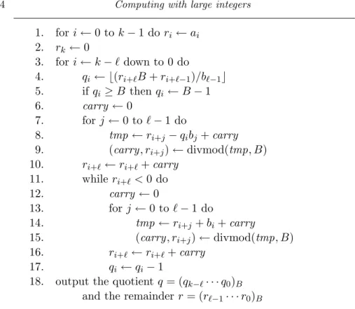
Based on this theorem, we first present an algorithm for division with re- mainder that works assuming thatbis appropriately “normalized,” meaning thatb`−1 ≥2w−1, whereB = 2w. This algorithm is shown in Fig. 3.1.
Some remarks are in order:
1. In line 4, we compute qi, which by Theorem 3.2 is greater than or equal to the true quotient digit, but exceeds this value by at most 2.
2. In line 5, we reduceqi if it is obviously too big.
3. In lines 6–10, we compute
(ri+`· · ·ri)B←(ri+`· · ·ri)B−qib.
In each loop iteration, the value oftmp lies between−(B2−B) and B−1, and the value carry lies between −(B−1) and 0.
4. If the estimate qi is too large, this is manifested by a negative value ofri+` at line 10. Lines 11–17 detect and correct this condition: the loop body here executes at most twice; in lines 12–16, we compute
(ri+`· · ·ri)B←(ri+`· · ·ri)B+ (b`−1· · ·b0)B.
Just as in the algorithm in§3.3.1, in every iteration of the loop in lines 13–15, the value ofcarry is 0 or 1, and the valuetmp lies between 0 and 2B−1.
It is quite easy to see that the running time of the above algorithm is O(`·(k−`+ 1)).
1. fori←0 to k−1 dori←ai 2. rk ←0
3. fori←k−`down to 0 do
4. qi ← b(ri+`B+ri+`−1)/b`−1c 5. ifqi ≥B thenqi←B−1 6. carry ←0
7. forj←0 to `−1 do
8. tmp ←ri+j−qibj+carry 9. (carry, ri+j)←divmod(tmp, B) 10. ri+`←ri+`+carry
11. while ri+`<0 do
12. carry ←0
13. forj ←0 to`−1 do
14. tmp←ri+j+bi+carry
15. (carry, ri+j)←divmod(tmp, B) 16. ri+`←ri+`+carry
17. qi←qi−1
18. output the quotientq = (qk−`· · ·q0)B
and the remainder r= (r`−1· · ·r0)B
Fig. 3.1. Division with Remainder Algorithm
Finally, consider the general case, where b may not be normalized. We multiply both a and b by an appropriate value 2w0, with 0 ≤ w0 < w, obtaining a0 :=a2w0 and b0 := 2w0, where b0 is normalized; alternatively, we can use a more efficient, special-purpose “left shift” algorithm to achieve the same effect. We then compute q and r0 such that a0 = b0q+r0, using the above division algorithm for the normalized case. Observe that q = ba0/b0c=ba/bc, and r0 =r2w0, where r=amodb. To recoverr, we simply divide r0 by 2w0, which we can do either using the above “single precision”
division algorithm, or by using a special-purpose “right shift” algorithm. All of this normalizing and denormalizing takes timeO(k+`). Thus, the total running time for division with remainder is still O(`·(k−`+ 1)).
Exercise3.14. Work out the details of algorithms for arithmetic onsigned integers, using the above algorithms for unsigned integers as subroutines.
You should give algorithms for addition, subtraction, multiplication, and
3.3 Basic integer arithmetic 45 division with remainder of arbitrary signed integers (for division with re- mainder, your algorithm should compute ba/bc and amodb). Make sure your algorithm correctly computes the sign bit of the result, and also strips leading zero digits from the result.
Exercise 3.15. Work out the details of an algorithm that compares two signed integers aand b, determining which ofa < b,a=b, ora > b holds.
Exercise3.16. Suppose that we run the division with remainder algorithm in Fig. 3.1 for ` > 1 without normalizing b, but instead, we compute the valueqi in line 4 as follows:
qi← b(ri+`B2+ri+`−1B+ri+`−2)/(b`−1B+b`−2)c.
Show that qi is either equal to the correct quotient digit, or the correct quotient digit plus 1. Note that a limitation of this approach is that the numbers involved in the computation are larger than B2.
Exercise 3.17. Work out the details for an algorithm that shifts a given unsigned integerato the left by a specified number of bitss(i.e., computes b := a·2s). The running time of your algorithm should be linear in the number of digits of the output.
Exercise 3.18. Work out the details for an algorithm that shifts a given unsigned integerato the right by a specified number of bitss(i.e., computes b := ba/2sc). The running time of your algorithm should be linear in the number of digits of the output. Now modify your algorithm so that it correctly computesba/2sc forsigned integers a.
Exercise 3.19. This exercise is for C/Java programmers. Evaluate the C/Java expressions
(-17) % 4; (-17) & 3;
and compare these values with (−17) mod 4. Also evaluate the C/Java expressions
(-17) / 4; (-17) >> 2;
and compare withb−17/4c. Explain your findings.
Exercise 3.20. This exercise is also for C/Java programmers. Suppose that values of typeintare stored using a 32-bit 2’s complement representa- tion, and that all basic arithmetic operations are computed correctly modulo 232, even if an “overflow” happens to occur. Also assume that double pre- cision floating point has 53 bits of precision, and that all basic arithmetic
operations give a result with a relative error of at most 2−53. Also assume that conversion from typeinttodoubleis exact, and that conversion from doubletointtruncates the fractional part. Now, suppose we are givenint variables a, b, and n, such that 1 < n< 230, 0 ≤ a < n, and 0 ≤ b < n.
Show that after the following code sequence is executed, the value of r is equal to (a·b) modn:
int q;
q = (int) ((((double) a) * ((double) b)) / ((double) n));
r = a*b - q*n;
if (r >= n) r = r - n;
else if (r < 0) r = r + n;
3.3.5 Summary
We now summarize the results of this section. For an integer a, we define len(a) to be the number of bits in the binary representation of |a|; more precisely,
len(a) :=
blog2|a|c+ 1 ifa6= 0,
1 ifa= 0.
Notice that fora >0, if `:= len(a), then we have log2a < `≤log2a+ 1, or equivalently, 2`−1 ≤a <2`.
Assuming that arbitrarily large integers are represented as described at the beginning of this section, with a sign bit and a vector of base-B digits, whereB is a constant power of 2, we may state the following theorem.
Theorem 3.3. Let aand b be arbitrary integers.
(i) We can compute a±b in time O(len(a) + len(b)).
(ii) We can compute a·bin time O(len(a) len(b)).
(iii) If b6= 0, we can compute the quotient q :=ba/bc and the remainder r:=amodb in time O(len(b) len(q)).
Note the boundO(len(b) len(q)) in part (iii) of this theorem, which may be significantly less than the boundO(len(a) len(b)). A good way to remember this bound is as follows: the time to compute the quotient and remainder is roughly the same as the time to compute the product bq appearing in the equalitya=bq+r.
This theorem does not explicitly refer to the base B in the underlying
3.3 Basic integer arithmetic 47 implementation. The choice of B affects the values of the implied big-O constants; while in theory, this is of no significance, it does have a significant impact in practice.
From now on, we shall (for the most part) not worry about the imple- mentation details of long-integer arithmetic, and will just refer directly this theorem. However, we will occasionally exploit some trivial aspects of our data structure for representing large integers. For example, it is clear that in constant time, we can determine the sign of a given integer a, the bit length of a, and any particular bit of the binary representation of a; more- over, as discussed in Exercises 3.17 and 3.18, multiplications and divisions by powers of 2 can be computed in linear time via “left shifts” and “right shifts.” It is also clear that we can convert between the base-2 representa- tion of a given integer and our implementation’s internal representation in linear time (other conversions may take longer — see Exercise 3.25).
A note on notation: “len” and “log.” In expressing the run- ning times of algorithms, we generally prefer to write, for exam- ple, O(len(a) len(b)), rather than O((loga)(logb)). There are two reasons for this. The first is esthetic: the function “len” stresses the fact that running times should be expressed in terms of the bit length of the inputs. The second is technical: big-O estimates in- volving expressions containing several independent parameters, like O(len(a) len(b)), should be valid forallpossible values of the param- eters, since the notion of “sufficiently large” does not make sense in this setting; because of this, it is very inconvenient to have functions, like log, that vanish or are undefined on some inputs.
Exercise 3.21. Letn1, . . . , nk be positive integers. Show that
k
X
i=1
len(ni)−k≤len k
Y
i=1
ni
≤
k
X
i=1
len(ni).
Exercise 3.22. Show that the product n of integers n1, . . . , nk, with each ni > 1, can be computed in time O(len(n)2). Do not assume that k is a constant.
Exercise 3.23. Show that given integers n1, . . . , nk, with eachni >1, and an integerz, where 0≤z < nandn:=Q
ini, we can compute thekintegers zmodni, fori= 1, . . . , k, in time O(len(n)2).
Exercise3.24. Consider the problem of computingbn1/2c for a given non- negative integern.
(a) Using binary search, give an algorithm for this problem that runs in
time O(len(n)3). Your algorithm should discover the bits of bn1/2c one at a time, from high- to low-order bit.
(b) Refine your algorithm from part (a), so that it runs in time O(len(n)2).
Exercise3.25. Show how to convert (in both directions) between the base- 10 representation and our implementation’s internal representation of an integernin time O(len(n)2).
3.4 Computing in Zn
Letn >1. Forα∈Zn, there exists a unique integera∈ {0, . . . , n−1}such that α = [a]n; we call this integer athe canonical representative of α, and denote it by rep(α). For computational purposes, we represent elements ofZn by their canonical representatives.
Addition and subtraction in Zn can be performed in time O(len(n)):
given α, β ∈ Zn, to compute rep(α+β), we simply compute the integer sum rep(α) + rep(β), subtracting n if the result is greater than or equal to n; similarly, to compute rep(α−β), we compute the integer difference rep(α)−rep(β), addingnif the result is negative. Multiplication in Zncan be performed in timeO(len(n)2): givenα, β ∈Zn, we compute rep(α·β) as rep(α) rep(β) modn, using one integer multiplication and one division with remainder.
A note on notation: “rep,” “mod,” and “[·]n.” In describ- ing algorithms, as well as in other contexts, ifα, β are elements of Zn, we may write, for example, γ ← α+β or γ ← αβ, and it is understood that elements ofZn are represented by their canonical representatives as discussed above, and arithmetic on canonical rep- resentatives is done modulo n. Thus, we have in mind a “strongly typed” language for our pseudo-code that makes a clear distinction between integers in the set {0, . . . , n−1} and elements of Zn. If a∈Z, we can convertato an object α∈Zn by writing α←[a]n, and ifa∈ {0, . . . , n−1}, this type conversion is purely conceptual, involving no actual computation. Conversely, ifα∈Zn, we can con- vertαto an objecta∈ {0, . . . , n−1}, by writinga←rep(α); again, this type conversion is purely conceptual, and involves no actual computation. It is perhaps also worthwhile to stress the distinction between amodn and [a]n— the former denotes an element of the set{0, . . . , n−1}, while the latter denotes an element ofZn.
Another interesting problem is exponentiation in Zn: given α ∈ Zn and a non-negative integer e, compute αe ∈ Zn. Perhaps the most obvious way to do this is to iteratively multiply by α a total of e times, requiring
3.4 Computing inZn 49 timeO(elen(n)2). A much faster algorithm, therepeated-squaring algo- rithm, computes αe using just O(len(e)) multiplications inZn, thus taking timeO(len(e) len(n)2).
This method works as follows. Lete= (b`−1· · ·b0)2 be the binary expan- sion ofe(whereb0 is the low-order bit). Fori= 0, . . . , `, defineei :=be/2ic;
the binary expansion of ei is ei = (b`−1· · ·bi)2. Also define βi := αei for i= 0, . . . , `, soβ`= 1 and β0 =αe. Then we have
ei= 2ei+1+bi and βi =βi+12 ·αbi fori= 0, . . . , `−1.
This idea yields the following algorithm:
β←[1]n
fori←`−1 down to 0 do β ←β2
ifbi = 1 thenβ←β·α outputβ
It is clear that when this algorithm terminates, we have β=αe, and that the running-time estimate is as claimed above. Indeed, the algorithm uses
`squarings in Zn, and at most `additional multiplications in Zn.
The following exercises develop some important efficiency improvements to the basic repeated-squaring algorithm.
Exercise 3.26. The goal of this exercise is to develop a “2t-ary” variant of the above repeated-squaring algorithm, in which the exponent is effectively treated as a number in base 2t, rather than in base 2.
(a) Show how to modify the repeated squaring so as to computeαeusing
`+O(1) squarings inZn, and an additional 2t+`/t+O(1) multiplica- tions inZn. As above, α∈Zn and len(e) =`, while tis a parameter that we are free to choose. Your algorithm should begin by building a table of powers [1], α, . . . , α2t−1, and after that, it should process the bits of e from left to right in blocks of length t (i.e., as base-2t digits).
(b) Show that by appropriately choosing the parametert, we can bound the number of additional multiplications inZnbyO(`/len(`)). Thus, from an asymptotic point of view, the cost of exponentiation is es- sentially the cost of`squarings in Zn.
(c) Improve your algorithm from part (a), so that it only uses `+O(1) squarings inZn, and an additional 2t−1+`/t+O(1) multiplications
in Zn. Hint: build a table that contains only the odd powers of α among [1], α, . . . , α2t−1.
Exercise 3.27. Suppose we are given α1, . . . , αk ∈ Zn, along with non- negative integerse1, . . . , ek, where len(ei)≤`fori= 1, . . . , k. Show how to compute
β :=α1e1· · ·αekk
using `+O(1) squarings inZn and an additional`+ 2k+O(1) multiplica- tions in Zn. Your algorithm should work in two phases: in the first phase, the algorithm uses just the valuesα1, . . . , αk to build a table of all possible products of subsets of α1, . . . , αk; in the second phase, the algorithm com- putesβ, using the exponents e1, . . . , ek, and the table computed in the first phase.
Exercise 3.28. Suppose that we are to compute αe, where α ∈ Zn, for many`-bit exponentse, but withαfixed. Show that for any positive integer parameter k, we can make a pre-computation (depending on α, `, and k) that uses`+O(1) squarings inZn and 2k+O(1) multiplications inZn, so that after the pre-computation, we can computeαefor any`-bit exponente using just`/k+O(1) squarings and`/k+O(1) multiplications inZn. Hint:
use the algorithm in the previous exercise.
Exercise3.29. Letkbe aconstant, positive integer. Suppose we are given α1, . . . , αk∈Zn, along with non-negative integerse1, . . . , ek, where len(ei)≤
`fori= 1, . . . , k. Show how to compute β :=α1e1· · ·αekk
using`+O(1) squarings inZnand an additionalO(`/len(`)) multiplications inZn. Hint: develop a 2t-ary version of the algorithm in Exercise 3.27.
Exercise 3.30. Let m1, . . . , mr be integers, each greater than 1, and let m :=m1· · ·mr. Also, for i= 1, . . . , r, define m0i := m/mi. Given α∈ Zn, show how to compute all of the quantities
αm01, . . . , αm0r
using a total of O(len(r) len(m)) multiplications in Zn. Hint: divide and conquer.
Exercise 3.31. The repeated-squaring algorithm we have presented here processes the bits of the exponent from left to right (i.e., from high order to low order). Develop an algorithm for exponentiation in Zn with similar complexity that processes the bits of the exponent from right to left.
3.5 Faster integer arithmetic (∗) 51 3.5 Faster integer arithmetic (∗)
The quadratic-time algorithms presented in §3.3 for integer multiplication and division are by no means the fastest possible. The next exercise develops a faster multiplication algorithm.
Exercise 3.32. Suppose we have two positive, `-bit integers a and b such that a=a12k+a0 and b=b12k+b0, where 0 ≤a0 <2k and 0≤b0 <2k. Then
ab=a1b122k+ (a0b1+a1b0)2k+a0b0.
Show how to compute the productabin time O(`), given the productsa0b0, a1b1, and (a0−a1)(b0 −b1). From this, design a recursive algorithm that computes abin timeO(`log23). (Note that log23≈1.58.)
The algorithm in the previous is also not the best possible. In fact, it is possible to multiply `-bit integers on a RAM in time O(`), but we do not explore this any further here (see§3.6).
The following exercises explore the relationship between integer multipli- cation and related problems. We assume that we have an algorithm that multiplies two integers of at most`bits in timeM(`). It is convenient (and reasonable) to assume that M is a well-behaved complexity function.
By this, we mean thatM maps positive integers to positive real numbers, and
• for all positive integersa and b, we have M(a+b)≥M(a) +M(b), and
• for all real c > 1 there exists real d > 1, such that for all positive integersa andb, ifa≤cb, thenM(a)≤dM(b).
Exercise 3.33. Let α > 0, β ≥ 1, γ ≥ 0, δ ≥ 0 be real constants. Show that
M(`) :=α`βlen(`)γlen(len(`))δ is a well-behaved complexity function.
Exercise 3.34. Give an algorithm for Exercise 3.22 that runs in time O(M(len(n)) len(k)).
Hint: divide and conquer.
Exercise 3.35. We can represent a “floating point” number ˆz as a pair (a, e), where a and e are integers — the value of ˆz is the rational number
a2e, and we call len(a) the precision of ˆz. We say that ˆz is a k-bit ap- proximation of a real number z if ˆz has precision k and ˆz = (1 +)z for some || ≤ 2−k+1. Show how to compute — given positive integers b and k— a k-bit approximation of 1/b in time O(M(k)). Hint: using Newton iteration, show how to go from a t-bit approximation of 1/b to a (2t−2)- bit approximation of 1/b, making use of just the high-order O(t) bits of b, in time O(M(t)). Newton iteration is a general method of iteratively approximating a root of an equationf(x) = 0 by starting with an initial ap- proximation x0, and computing subsequent approximations by the formula xi+1 = xi −f(xi)/f0(xi), where f0(x) is the derivative of f(x). For this exercise, apply Newton iteration to the functionf(x) =x−1−b.
Exercise 3.36. Using the result of the previous exercise, given positive integers a and b of bit length at most `, show how to compute ba/bc and amodb in time O(M(`)). From this, we see that up to a constant factor, division with remainder is no harder that multiplication.
Exercise 3.37. Using the result of the previous exercise, give an algorithm for Exercise 3.23 that runs in time O(M(len(n)) len(k)). Hint: divide and conquer.
Exercise 3.38. Give an algorithm for Exercise 3.24 that runs in time O(M(len(n))). Hint: Newton iteration.
Exercise 3.39. Give algorithms for Exercise 3.25 that run in time O(M(`) len(`)), where`:= len(n). Hint: divide and conquer.
Exercise3.40. Suppose we have an algorithm that computes the square of an`-bit integer in timeS(`), whereS is a well-behaved complexity function.
Show how to use this algorithm to compute the product of two arbitrary integers of at most`bits in time O(S(`)).
3.6 Notes
Shamir [84] shows how to factor an integer in polynomial time on a RAM, but where the numbers stored in the memory cells may have exponentially many bits. As there is no known polynomial-time factoring algorithm on any realistic machine, Shamir’s algorithm demonstrates the importance of restricting the sizes of numbers stored in the memory cells of our RAMs to keep our formal model realistic.
The most practical implementations of algorithms for arithmetic on large
3.6 Notes 53 integers are written in low-level “assembly language,” specific to a partic- ular machine’s architecture (e.g., the GNU Multi-Precision library GMP, available at www.swox.com/gmp). Besides the general fact that such hand- crafted code is more efficient than that produced by a compiler, there is another, more important reason for using such code. A typical 32-bit ma- chine often comes with instructions that allow one to compute the 64-bit product of two 32-bit integers, and similarly, instructions to divide a 64-bit integer by a 32-bit integer (obtaining both the quotient and remainder).
However, high-level programming languages do not (as a rule) provide any access to these low-level instructions. Indeed, we suggested in§3.3 using a value for the base B of about half the word-size of the machine, so as to avoid overflow. However, if one codes in assembly language, one can takeB to be much closer to, or even equal to, the word-size of the machine. Since our basic algorithms for multiplication and division run in time quadratic in the number of base-B digits, the effect of doubling the bit-length ofB is to decrease the running time of these algorithms by a factor of four. This effect, combined with the improvements one might typically expect from us- ing assembly-language code, can easily lead to a five- to ten-fold decrease in the running time, compared to an implementation in a high-level language.
This is, of course, a significant improvement for those interested in serious
“number crunching.”
The “classical,” quadratic-time algorithms presented here for integer mul- tiplication and division are by no means the best possible: there are algo- rithms that are asymptotically faster. We saw this in the algorithm in Exercise 3.32, which was originally invented by Karatsuba [52] (although Karatsuba is one of two authors on this paper, the paper gives exclusive credit for this particular result to Karatsuba). That algorithm allows us to multiply two `-bit integers in timeO(`log23). The fastest known algorithm for multiplying two`-bit integers on a RAM runs in time O(`). This algo- rithm is due to Sch¨onhage, and actually works on a very restricted type of RAM called a “pointer machine” (see Problem 12, Section 4.3.3 of Knuth [54]). See Exercise 18.27 later in this text for a much simpler (but heuristic) O(`) multiplication algorithm.
Another model of computation is that ofBoolean circuits. In this model of computation, one considers families of Boolean circuits (with, say, the usual “and,” “or,” and “not” gates) that compute a particular function — for every input length, there is a different circuit in the family that computes the function on inputs of that length. One natural notion of complexity for such circuit families is thesizeof the circuit (i.e., the number of gates and
wires in the circuit), which is measured as a function of the input length.
The smallest known Boolean circuit that multiplies two `-bit numbers has sizeO(`len(`) len(len(`))). This result is due to Sch¨onhage and Strassen [82].
It is hard to say which model of computation, the RAM or circuits, is
“better.” On the one hand, the RAM very naturally models computers as we know them today: one stores small numbers, like array indices, coun- ters, and pointers, in individual words of the machine, and processing such a number typically takes a single “machine cycle.” On the other hand, the RAM model, as we formally defined it, invites a certain kind of “cheating,”
as it allows one to stuffO(len(`))-bit integers into memory cells. For exam- ple, even with the simple, quadratic-time algorithms for integer arithmetic discussed in §3.3, we can choose the base B to have len(`) bits, in which case these algorithms would run in time O((`/len(`))2). However, just to keep things simple, we have chosen to viewB as a constant (from a formal, asymptotic point of view).
In the remainder of this text, unless otherwise specified, we shall always use the classicalO(`2) bounds for integer multiplication and division, which have the advantage of being both simple and reasonably reliable predictors of actual performance for small to moderately sized inputs. For relatively large numbers, experience shows that the classical algorithms are definitely not the best — Karatsuba’s multiplication algorithm, and related algorithms for division, start to perform significantly better than the classical algorithms on inputs of a thousand bits or so (the exact crossover depends on myriad implementation details). The even “faster” algorithms discussed above are typically not interesting unless the numbers involved are truly huge, of bit length around 105–106. Thus, the reader should bear in mind that for serious computations involving very large numbers, the faster algorithms are very important, even though this text does not discuss them at great length.
For a good survey of asymptotically fast algorithms for integer arithmetic, see Chapter 9 of Crandall and Pomerance [30], as well as Chapter 4 of Knuth [54].