What do this week’s weather forecast and organization performance have in common?
Most of the time, reality doesn’t match expectations. Cloudy skies that cancel a little league game may suddenly let the sun shine through just as the vans are packed. Jubilant business owners may change their tune when they tally their monthly bills and discover that skyrocketing operation costs have significantly reduced their profits. Differences, or variances, are all around us.
For organizations, variances are of great value because they highlight the areas where performance most lags expectations. By using this information to make corrective adjustments, companies can achieve significant savings, as the following article shows.
Overhead Cost Variances Force Macy’s to Shop for Changes in Strategy 1
Managers frequently review the differences, or variances, in overhead costs and make changes in the operations of a business. Sometimes staffing levels are increased or decreased, while at other times managers identify ways to use fewer resources like, say, office supplies and travel for business meetings that don’t add value to the products and services that customers buy.
At the department-store chain Macy’s, however, managers analyzed overhead cost variances and changed the way the company purchased the products it sells. In 2005, when Federated Department Stores and the May Department Store Company merged, Macy’s operated seven buying offices across the United States. Each of these offices was responsible for purchasing some of the clothes, cosmetics, jewelry, and many other items Macy’s sells. But overlapping responsibilities, seasonal buying patterns (clothes are generally purchased in the spring and fall) and regional differences in costs and salaries (for example, it costs more for employees and rent in San Francisco than Cincinnati) led to frequent and significant variances in overhead costs.
These overhead costs weighed on the company as the retailer struggled with disappointing sales after the merger. As a result,
Macy’s leaders felt pressured to reduce its costs that were not directly related to selling merchandise in stores and online.
8
Learning Objectives
1. Explain the similarities and differ- ences in planning variable overhead costs and fixed overhead costs
2. Develop budgeted variable over- head cost rates and budgeted fixed overhead cost rates
3. Compute the variable overhead flexible-budget variance, the vari- able overhead efficiency variance, and the variable overhead spend- ing variance
4. Compute the fixed overhead flexible-budget variance, the fixed overhead spending variance, and the fixed overhead production- volume variance
5. Show how the 4-variance analysis approach reconciles the actual overhead incurred with the over- head amounts allocated during the period
6. Explain the relationship between the sales-volume variance and the production-volume variance
7. Calculate overhead variances in activity-based costing
8. Examine the use of overhead vari- ances in nonmanufacturing settings
䉲
Flexible Budgets, Overhead Cost
Variances, and Management Control
1Sources: Boyle, Matthew. 2009. A leaner Macy’s tries to cater to local tastes. BusinessWeek.com, September 3;
Kapner, Suzanne. 2009. Macy’s looking to cut costs. Fortune, January 14. http://money.cnn.com/2009/01/14/news/
companies/macys_consolidation.fortune/;Macy’s 2009 Corporate Fact Book. 2009. Cincinnati: Macy’s, Inc., 7.
262
network of seven buying offices into one location in New York. With all centralized buying and merchandise planning in one location, Macy’s buying structure and overhead costs were in line with how many other large chains operate, including JCPenney and Kohl’s. All told, the move to centralized buying
would generate $100 million in annualized cost savings for the company.
While centralized buying was applauded by industry experts and shareholders, Macy’s CEO Terry Lundgren was concerned about keeping a “localized flavor” in his stores. To ensure that nationwide buying accommodated local tastes, a new team of merchants was formed in each Macy’s market to gauge local buying habits. That way, the company could reduce its overhead costs while ensuring that Macy’s stores near water parks had extra swimsuits.
Companies such as DuPont, International Paper, and U.S. Steel, which invest heavily in capital
equipment, or Amazon.com and Yahoo!, which invest large amounts in software, have high overhead costs.
As the Macy’s example suggests, understanding the behavior of overhead costs, planning for them, performing variance analysis, and acting appropriately on the results are critical for a company.
In this chapter, we will examine how flexible budgets and variance analysis can help managers plan and control overhead costs.
Chapter 7 emphasized the direct-cost categories of direct materials and direct manufacturing labor. In this chapter, we focus on the indirect-cost categories of variable manufacturing overhead and fixed manufacturing overhead. Finally, we explain why managers should be careful when interpreting variances based on overhead-cost concepts developed primarily for financial reporting purposes.
Planning of Variable and Fixed Overhead Costs
We’ll use the Webb Company example again to illustrate the planning and control of vari- able and fixed overhead costs. Recall that Webb manufactures jackets that are sold to dis- tributors who in turn sell to independent clothing stores and retail chains. For simplicity, we assume Webb’s only costs are manufacturingcosts. For ease of exposition, we use the term overhead costs instead of manufacturing overhead costs. Variable (manufacturing) overhead costs for Webb include energy, machine maintenance, engineering support, and indirect materials. Fixed (manufacturing) overhead costs include plant leasing costs, depreciation on plant equipment, and the salaries of the plant managers.
Learning Objective 1
Explain the similarities and differences in planning variable overhead costs and fixed overhead costs . . . for both, plan only essential activities and be efficient; fixed overhead costs are usually determined well before the budget period begins
Planning Variable Overhead Costs
To effectively plan variable overhead costs for a product or service, managers must focus attention on the activities that create a superior product or service for their customers and eliminate activities that do not add value. Webb’s managers examine how each of their variable overhead costs relates to delivering a superior product or service to cus- tomers. For example, customers expect Webb’s jackets to last, so managers at Webb con- sider sewing to be an essential activity. Therefore, maintenance activities for sewing machines—included in Webb’s variable overhead costs—are also essential activities for which management must plan. In addition, such maintenance should be done in a cost- effective way, such as by scheduling periodic equipment maintenance rather than waiting for sewing machines to break down. For many companies today, it is critical to plan for ways to become more efficient in the use of energy, a rapidly growing component of vari- able overhead costs. Webb installs smart meters in order to monitor energy use in real time and steer production operations away from peak consumption periods.
Planning Fixed Overhead Costs
Effective planning of fixed overhead costs is similar to effective planning for variable overhead costs—planning to undertake only essential activities and then planning to be efficient in that undertaking. But in planning fixed overhead costs, there is one more strategic issue that managers must take into consideration: choosing the appropriate level of capacity or investment that will benefit the company in the long run. Consider Webb’s leasing of sewing machines, each having a fixed cost per year. Leasing more machines than necessary—if Webb overestimates demand—will result in additional fixed leasing costs on machines not fully used during the year. Leasing insufficient machine capacity—say, because Webb underestimates demand or because of limited space in the plant—will result in an inability to meet demand, lost sales of jackets, and unhappy customers. Consider the example of AT&T, which did not foresee the iPhone’s appeal or the proliferation of “apps” and did not upgrade its network sufficiently to handle the resulting data traffic. AT&T has since had to impose limits on how cus- tomers can use the iPhone (such as by curtailing tethering and the streaming of Webcasts). In December 2009, AT&T had the lowest customer satisfaction ratings among all major carriers.
The planning of fixed overhead costs differs from the planning of variable overhead costs in one important respect: timing. At the start of a budget period, management will have made most of the decisions that determine the level of fixed overhead costs to be incurred. But, it’s the day-to-day, ongoing operating decisions that mainly determine the level of variable overhead costs incurred in that period. In health care settings, for exam- ple, variable overhead, which includes disposable supplies, unit doses of medication, suture packets, and medical waste disposal costs, is a function of the number and nature of procedures carried out, as well as the practice patterns of the physicians. However, the majority of the cost of providing hospital service is related to buildings, equipment, and salaried labor, which are fixed overhead items, unrelated to the volume of activity.2
Standard Costing at Webb Company
Webb uses standard costing. The development of standards for Webb’s direct manufac- turing costs was described in Chapter 7. This chapter discusses the development of stan- dards for Webb’s manufacturing overhead costs. Standard costing is a costing system that (a) traces direct costs to output produced by multiplying the standard prices or rates by the standard quantities of inputs allowed for actual outputs produced and (b) allo- cates overhead costs on the basis of the standard overhead-cost rates times the standard quantities of the allocation bases allowed for the actual outputs produced.
2Related to this, free-standing surgery centers have thrived because they have an economic advantage of lower fixed overhead when compared to a traditional hospital. For an enlightening summary of costing issues in health care, see A. Macario, “What Does One Minute of Operating Room Time Cost?” Stanford University School of Medicine (2009).
Learning Objective 2
Develop budgeted variable overhead cost rates
. . . budgeted variable costs divided by quantity of cost-allocation base and budgeted fixed overhead cost rates . . . budgeted fixed costs divided by quantity of cost-allocation base
Decision Point
How do managers plan variable overhead costs and fixed overhead costs?
The standard cost of Webb’s jackets can be computed at the start of the budget period.
This feature of standard costing simplifies record keeping because no record is needed of the actual overhead costs or of the actual quantities of the cost-allocation bases used for mak- ing the jackets. What is needed are the standard overhead cost rates for variable and fixed overhead. Webb’s management accountants calculate these cost rates based on the planned amounts of variable and fixed overhead and the standard quantities of the allocation bases.
We describe these computations next. Note that once standards have been set, the costs of using standard costing are low relative to the costs of using actual costing or normal costing.
Developing Budgeted Variable Overhead Rates
Budgeted variable overhead cost-allocation rates can be developed in four steps. We use the Webb example to illustrate these steps. Throughout the chapter, we use the broader term
“budgeted rate” rather than “standard rate” to be consistent with the term used in describing normal costing in earlier chapters. In standard costing, the budgeted rates are standard rates.
Step 1: Choose the Period to Be Used for the Budget.Webb uses a 12-month budget period. Chapter 4 (p. 103) provides two reasons for using annual overhead rates rather than, say, monthly rates. The first relates to the numerator (such as reducing the influence of seasonality on the cost structure) and the second to the denominator (such as reducing the effect of varying output and number of days in a month). In addition, setting overhead rates once a year saves management the time it would need 12 times during the year if budget rates had to be set monthly.
Step 2: Select the Cost-Allocation Bases to Use in Allocating Variable Overhead Costs to Output Produced.Webb’s operating managers select machine-hours as the cost-allocation base because they believe that machine-hours is the only cost driver of variable overhead.
Based on an engineering study, Webb estimates it will take 0.40 of a machine-hour per actual output unit. For its budgeted output of 144,000 jackets in 2011, Webb budgets 57,600 (0.40 144,000) machine-hours.
Step 3: Identify the Variable Overhead Costs Associated with Each Cost-Allocation Base.
Webb groups all of its variable overhead costs, including costs of energy, machine mainte- nance, engineering support, indirect materials, and indirect manufacturing labor in a single cost pool. Webb’s total budgeted variable overhead costs for 2011 are $1,728,000.
Step 4: Compute the Rate per Unit of Each Cost-Allocation Base Used to Allocate Variable Overhead Costs to Output Produced.Dividing the amount in Step 3 ($1,728,000) by the amount in Step 2 (57,600 machine-hours), Webb estimates a rate of $30 per stan- dard machine-hour for allocating its variable overhead costs.
In standard costing, the variable overhead rate per unit of the cost-allocation base ($30 per machine-hour for Webb) is generally expressed as a standard rate per output unit. Webb calculates the budgeted variable overhead cost rate per output unit as follows:
Webb uses $12 per jacket as the budgeted variable overhead cost rate in both its static budget for 2011 and in the monthly performance reports it prepares during 2011.
The $12 per jacket represents the amount by which Webb’s variable overhead costs are expected to change with respect to output units for planning and control purposes.
Accordingly, as the number of jackets manufactured increases, variable overhead costs are allocated to output units (for the inventory costing purpose) at the same rate of $12 per jacket. Of course, this presents an overall picture of total variable overhead costs, which in reality consist of many items, including energy, repairs, indirect labor, and so on.
Managers help control variable overhead costs by budgeting each line item and then investigating possible causes for any significant variances.
= $12 per jacket
= 0.40 hour per jacket * $30 per hour Budgeted variable Budgeted input Budgeted variable overhead cost rate = allowed per * overhead cost rate
per output unit output unit per input unit
*
Developing Budgeted Fixed Overhead Rates
Fixed overhead costs are, by definition, a lump sum of costs that remains unchanged in total for a given period, despite wide changes in the level of total activity or volume related to those overhead costs. Fixed costs are included in flexible budgets, but they remain the same total amount within the relevant range of activity regardless of the out- put level chosen to “flex” the variable costs and revenues. Recall from Exhibit 7-2, page 231 and the steps in developing a flexible budget, that the fixed-cost amount is the same $276,000 in the static budget and in the flexible budget. Do not assume, however, that fixed overhead costs can never be changed. Managers can reduce fixed overhead costs by selling equipment or by laying off employees. But they are fixed in the sense that, unlike variable costs such as direct material costs, fixed costs do not automatically increase or decrease with the level of activity within the relevant range.
The process of developing the budgeted fixed overhead rate is the same as that detailed earlier for calculating the budgeted variable overhead rate. The four steps are as follows:
Step 1: Choose the Period to Use for the Budget.As with variable overhead costs, the budget period for fixed overhead costs is typically 12 months to help smooth out seasonal effects.
Step 2: Select the Cost-Allocation Bases to Use in Allocating Fixed Overhead Costs to Output Produced.Webb uses machine-hours as the only cost-allocation base for fixed overhead costs. Why? Because Webb’s managers believe that, in the long run, fixed over- head costs will increase or decrease to the levels needed to support the amount of machine-hours. Therefore, in the long run, the amount of machine-hours used is the only cost driver of fixed overhead costs. The number of machine-hours is the denominator in the budgeted fixed overhead rate computation and is called the denominator levelor, in manufacturing settings, the production-denominator level. For simplicity, we assume Webb expects to operate at capacity in fiscal year 2011—with a budgeted usage of 57,600 machine-hours for a budgeted output of 144,000 jackets.3
Step 3: Identify the Fixed Overhead Costs Associated with Each Cost-Allocation Base.
Because Webb identifies only a single cost-allocation base—machine-hours—to allocate fixed overhead costs, it groups all such costs into a single cost pool. Costs in this pool include depreciation on plant and equipment, plant and equipment leasing costs, and the plant manager’s salary. Webb’s fixed overhead budget for 2011 is $3,312,000.
Step 4: Compute the Rate per Unit of Each Cost-Allocation Base Used to Allocate Fixed Overhead Costs to Output Produced.Dividing the $3,312,000 from Step 3 by the 57,600 machine-hours from Step 2, Webb estimates a fixed overhead cost rate of
$57.50 per machine-hour:
In standard costing, the $57.50 fixed overhead cost per machine-hour is usually expressed as a standard cost per output unit. Recall that Webb’s engineering study estimates that it will take 0.40 machine-hour per output unit. Webb can now calculate the budgeted fixed overhead cost per output unit as follows:
= $23.00 per jacket
= 0.40 of a machine-hour per jacket * $57.50 per machine-hour Budgeted fixed
overhead cost per output unit
=
Budgeted quantity of cost-allocation base allowed per
output unit
*
Budgeted fixed overhead cost
per unit of cost-allocation base Budgeted fixed
overhead cost per unit of cost-allocation
base
=
Budgeted total costs in fixed overhead cost pool
Budgeted total quantity of cost-allocation base
= $3,312,000
57,600 = $57.50 per machine-hour
3Because Webb plans its capacity over multiple periods, anticipated demand in 2011 could be such that budgeted output for 2011 is less than capacity. Companies vary in the denominator levels they choose; some may choose budgeted output and oth- ers may choose capacity. In either case, the basic approach and analysis presented in this chapter is unchanged. Chapter 9 dis- cusses choosing a denominator level and its implications in more detail.
When preparing monthly budgets for 2011, Webb divides the $3,312,000 annual total fixed costs into 12 equal monthly amounts of $276,000.
Variable Overhead Cost Variances
We now illustrate how the budgeted variable overhead rate is used in computing Webb’s variable overhead cost variances. The following data are for April 2011, when Webb produced and sold 10,000 jackets:
Actual Result Flexible-Budget Amount
1. Output units (jackets) 10,000 10,000
2. Machine-hours per output unit 0.45 0.40
3. Machine-hours (1 * 2) 4,500 4,000
4. Variable overhead costs $130,500 $120,000
5. Variable overhead costs per machine-hour (4 ÷ 3) $ 29.00 $ 30.00 6. Variable overhead costs per output unit (4 ÷ 1) $ 13.05 $ 12.00
Decision Point
How are budgeted variable overhead and fixed overhead cost rates calculated?
Learning Objective 3
Compute the variable overhead flexible- budget variance, . . . difference between actual variable overhead costs and flexible-budget variable overhead amounts the variable overhead efficiency variance, . . . difference between actual quantity of cost- allocation base and budgeted quantity of cost-allocation base and the variable overhead spending variance
. . . difference between actual variable overhead cost rate and budgeted variable overhead cost rate
As we saw in Chapter 7, the flexible budget enables Webb to highlight the differences between actual costs and actual quantities versus budgeted costs and budgeted quantities for the actual output level of 10,000 jackets.
Flexible-Budget Analysis
Thevariable overhead flexible-budget variancemeasures the difference between actual variable overhead costs incurred and flexible-budget variable overhead amounts.
This $10,500 unfavorable flexible-budget variance means Webb’s actual variable over- head exceeded the flexible-budget amount by $10,500 for the 10,000 jackets actually produced and sold. Webb’s managers would want to know why actual costs exceeded the flexible-budget amount. Did Webb use more machine-hours than planned to produce the 10,000 jackets? If so, was it because workers were less skilled than expected in using machines? Or did Webb spend more on variable overhead costs, such as maintenance?
Just as we illustrated in Chapter 7 with the flexible-budget variance for direct-cost items, Webb’s managers can get further insight into the reason for the $10,500 unfavor- able variance by subdividing it into the efficiency variance and spending variance.
Variable Overhead Efficiency Variance
Thevariable overhead efficiency varianceis the difference between actual quantity of the cost-allocation base used and budgeted quantity of the cost-allocation base that should have been used to produce actual output, multiplied by budgeted variable overhead cost per unit of the cost-allocation base.
= $15,000 U
= (4,500 hours - 4,000 hours) * $30 per hour
= (4,500 hours - 0.40 hr.>unit * 10,000 units) * $30 per hour Variable
overhead efficiency variance
= •
Actual quantity of variable overhead cost-allocation base
used for actual output
-
Budgeted quantity of variable overhead cost-allocation base
allowed for actual output
μ *
Budgeted variable overhead cost per unit of cost-allocation base
= $10,500 U
= $130,500- $120,000 Variable overhead
flexible-budget variance = Actual costs
incurred - Flexible-budget amount
Columns 2 and 3 of Exhibit 8-1 depict the variable overhead efficiency variance. Note the variance arises solely because of the difference between actual quantity (4,500 hours) and budgeted quantity (4,000 hours) of the cost-allocation base. The variable overhead effi- ciency variance is computed the same way the efficiency variance for direct-cost items is (Chapter 7, pp. 236–239). However, the interpretation of the variance is quite different.
Efficiency variances for direct-cost items are based on differences between actual inputs used and budgeted inputs allowed for actual output produced. For example, a forensic laboratory (the kind popularized by television shows such as CSIandDexter) would calculate a direct labor efficiency variance based on whether the lab used more or fewer hours than the stan- dard hours allowed for the actual number of DNA tests. In contrast, the efficiency variance for variable overhead cost is based on the efficiency with which the cost-allocation baseis used. Webb’s unfavorable variable overhead efficiency variance of $15,000 means that the actual machine-hours (the cost-allocation base) of 4,500 hours turned out to be higher than the budgeted machine-hours of 4,000 hours allowed to manufacture 10,000 jackets.
The following table shows possible causes for Webb’s actual machine-hours exceeding budgeted machine-hours and management’s potential responses to each of these causes.
Management would assess the cause(s) of the $15,000 U variance in April 2011 and respond accordingly. Note how, depending on the cause(s) of the variance, corrective actions may need to be taken not just in manufacturing but also in other business func- tions of the value chain, such as sales and distribution.
Flexible Budget:
Actual Costs Incurred:
Actual Input Quantity Actual Rate
Actual Input Quantity Budgeted Rate
Budgeted Input Quantity Allowed for Actual Output Budgeted Rate
(1) (2) (3)
(0.40 hr./unit 10,000 units $30/hr.) (4,500 hrs. $29/hr.)
$130,500
(4,500 hrs. $30/hr.) 4,000 hrs. $30/hr.
$135,000 $120,000
Level 3 $4,500 F $15,000 U
Spending variance Efficiency variance
Level 2 $10,500 U
Flexible-budget variance
aF favorable effect on operating income; U unfavorable effect on operating income.
Exhibit 8-1 Columnar Presentation of Variable Overhead Variance Analysis: Webb Company for April 2011a Possible Causes for Exceeding Budget Potential Management Responses 1. Workers were less skilled than expected in
using machines.
2. Production scheduler inefficiently scheduled jobs, resulting in more machine-hours used than budgeted.
3. Machines were not maintained in good operating condition.
4. Webb’s sales staff promised a distributor a rush delivery, which resulted in more machine-hours used than budgeted.
5. Budgeted machine time standards were set too tight.
1. Encourage the human resources department to implement better employee-hiring practices and training procedures.
2. Improve plant operations by installing production scheduling software.
3. Ensure preventive maintenance is done on all machines.
4. Coordinate production schedules with sales staff and distributors and share information with them.
5. Commit more resources to develop appropriate standards.
Webb’s managers discovered that one reason the machines operated below budgeted efficiency levels in April 2011 was insufficient maintenance performed in the prior two months. A former plant manager delayed maintenance in a presumed attempt to meet monthly budget cost targets. As we discussed in Chapter 6, managers should not be focused on meeting short-run budget targets if they are likely to result in harmful long-run consequences. Webb is now strengthening its internal maintenance procedures so that failure to do monthly maintenance as needed will raise a “red flag” that must be immedi- ately explained to management. Another reason for actual machine-hours exceeding bud- geted machine-hours was the use of underskilled workers. As a result, Webb is initiating steps to improve hiring and training practices.
Variable Overhead Spending Variance
Thevariable overhead spending varianceis the difference between actual variable over- head cost per unit of the cost-allocation base and budgeted variable overhead cost per unit of the cost-allocation base, multiplied by the actual quantity of variable overhead cost-allocation base used for actual output.
Since Webb operated in April 2011 with a lower-than-budgeted variable overhead cost per machine-hour, there is a favorable variable overhead spending variance. Columns 1 and 2 in Exhibit 8-1 depict this variance.
To understand the favorable variable overhead spending variance and its implica- tions, Webb’s managers need to recognize why actualvariable overhead cost per unit of the cost-allocation base ($29 per machine-hour) is lowerthan the budgetedvariable over- head cost per unit of the cost-allocation base ($30 per machine-hour). Overall, Webb used 4,500 machine-hours, which is 12.5% greater than the flexible-budget amount of 4,000 machine hours. However, actual variable overhead costs of $130,500 are only 8.75% greater than the flexible-budget amount of $120,000. Thus, relative to the flexible budget, the percentage increase in actual variable overhead costs is lessthan the percent- age increase in machine-hours. Consequently, actual variable overhead cost per machine- hour is lower than the budgeted amount, resulting in a favorable variable overhead spending variance.
Recall that variable overhead costs include costs of energy, machine maintenance, indi- rect materials, and indirect labor. Two possible reasons why the percentage increase in actual variable overhead costs is less than the percentage increase in machine-hours are as follows:
1. Actual prices of individual inputs included in variable overhead costs, such as the price of energy, indirect materials, or indirect labor, are lower than budgeted prices of these inputs. For example, the actual price of electricity may only be $0.09 per kilowatt- hour, compared with a price of $0.10 per kilowatt-hour in the flexible budget.
2. Relative to the flexible budget, the percentage increase in the actual usage of individual items in the variable overhead-cost pool is less than the percentage increase in machine- hours. Compared with the flexible-budget amount of 30,000 kilowatt-hours, suppose actual energy used is 32,400 kilowatt-hours, or 8% higher. The fact that this is a smaller percentage increase than the 12.5% increase in machine-hours (4,500 actual machine-hours versus a flexible budget of 4,000 machine hours) will lead to a favorable variable overhead spending variance. The favorable spending variance can be partially or completely traced to the efficient use of energy and other variable overhead items.
= $4,500 F
= (-$1 per machine-hour) * 4,500 machine-hours
= ($29 per machine-hour - $30 per machine-hour) * 4,500 machine-hours Variable
overhead spending variance
= §
Actual variable overhead cost per unit of cost-allocation base
-
Budgeted variable overhead cost per unit of cost-allocation base
¥ *
Actual quantity of variable overhead cost-allocation base used for actual output
As part of the last stage of the five-step decision-making process, Webb’s managers will need to examine the signals provided by the variable overhead variances to evaluate performance and learn. By understanding the reasons for these variances, Webb can take appropriate actions and make more precise predictions in order to achieve improved results in future periods.
For example, Webb’s managers must examine why actual prices of variable overhead cost items are different from budgeted prices. The price effects could be the result of skill- ful negotiation on the part of the purchasing manager, oversupply in the market, or lower quality of inputs such as indirect materials. Webb’s response depends on what is believed to be the cause of the variance. If the concerns are about quality, for instance, Webb may want to put in place new quality management systems.
Similarly, Webb’s managers should understand the possible causes for the efficiency with which variable overhead resources are used. These causes include skill levels of workers, maintenance of machines, and the efficiency of the manufacturing process.
Webb’s managers discovered that Webb used fewer supervision resources per machine- hour because of manufacturing process improvements. As a result, they began organizing crossfunctional teams to see if more process improvements could be achieved.
We emphasize that a favorable variable overhead spending variance is not always desir- able. For example, the variable overhead spending variance would be favorable if Webb’s managers purchased lower-priced, poor-quality indirect materials, hired less-talented super- visors, or performed less machine maintenance. These decisions, however, are likely to hurt product quality and harm the long-run prospects of the business.
To clarify the concepts of variable overhead efficiency variance and variable overhead spending variance, consider the following example. Suppose that (a) energy is the only item of variable overhead cost and machine-hours is the cost-allocation base; (b) actual machine-hours used equals the number of machine hours under the flexible budget; and (c) the actual price of energy equals the budgeted price. From (a) and (b), it follows that there is no efficiency variance — the company has been efficient with respect to the num- ber of machine-hours (the cost-allocation base) used to produce the actual output.
However, and despite (c), there could still be a spending variance. Why? Because even though the company used the correct number of machine hours, the energy consumed per machine hourcould be higher than budgeted (for example, because the machines have not been maintained correctly). The cost of this higher energy usage would be reflected in an unfavorable spending variance.
Journal Entries for Variable Overhead Costs and Variances
We now prepare journal entries for Variable Overhead Control and the contra account Variable Overhead Allocated.
Entries for variable overhead for April 2011 (data from Exhibit 8-1) are as follows:
1. Variable Overhead Control 130,500
Accounts Payable and various other accounts 130,500
To record actual variable overhead costs incurred.
2. Work-in-Process Control 120,000
Variable Overhead Allocated 120,000
To record variable overhead cost allocated
(0.40 machine-hour/unit 10,000 units $30/machine-hour). (The costs accumulated in Work-in-Process Control are transferred to Finished Goods Control when production is completed and to Cost of Goods Sold when the products are sold.)
*
*
3. Variable Overhead Allocated 120,000
Variable Overhead Efficiency Variance 15,000
Variable Overhead Control 130,500
Variable Overhead Spending Variance 4,500
To record variances for the accounting period.
These variances are the underallocated or overallocated variable overhead costs. At the end of the fiscal year, the variance accounts are written off to cost of goods sold if imma- terial in amount. If the variances are material in amount, they are prorated among Work- in-Process Control, Finished Goods Control, and Cost of Goods Sold on the basis of the variable overhead allocated to these accounts, as described in Chapter 4, pages 117–122.
As we discussed in Chapter 7, only unavoidable costs are prorated. Any part of the vari- ances attributable to avoidable inefficiency are written off in the period. Assume that the balances in the variable overhead variance accounts as of April 2011 are also the balances at the end of the 2011 fiscal year and are immaterial in amount. The following journal entry records the write-off of the variance accounts to cost of goods sold:
Cost of Goods Sold 10,500
Variable Overhead Spending Variance 4,500
Variable Overhead Efficiency Variance 15,000 We next consider fixed overhead cost variances.
Fixed Overhead Cost Variances
The flexible-budget amount for a fixed-cost item is also the amount included in the static budget prepared at the start of the period. No adjustment is required for differ- ences between actual output and budgeted output for fixed costs, because fixed costs are unaffected by changes in the output level within the relevant range. At the start of 2011, Webb budgeted fixed overhead costs to be $276,000 per month. The actual amount for April 2011 turned out to be $285,000. The fixed overhead flexible-budget varianceis the difference between actual fixed overhead costs and fixed overhead costs in the flexible budget:
The variance is unfavorable because $285,000 actual fixed overhead costs exceed the
$276,000 budgeted for April 2011, which decreases that month’s operating income by $9,000.
The variable overhead flexible-budget variance described earlier in this chapter was subdivided into a spending variance and an efficiency variance. There is not an efficiency variance for fixed overhead costs. That’s because a given lump sum of fixed overhead costs will be unaffected by how efficiently machine-hours are used to produce output in a given budget period. As we will see later on, this does not mean that a company cannot be efficient or inefficient in its use of fixed-overhead-cost resources. As Exhibit 8-2 shows, because there is no efficiency variance, the fixed overhead spending varianceis the same amount as the fixed overhead flexible-budget variance:
Reasons for the unfavorable spending variance could be higher plant-leasing costs, higher depreciation on plant and equipment, or higher administrative costs, such as a higher-than-budgeted salary paid to the plant manager. Webb investigated this variance and found that there was a $9,000 per month unexpected increase in its equipment- leasing costs. However, management concluded that the new lease rates were competi- tive with lease rates available elsewhere. If this were not the case, management would look to lease equipment from other suppliers.
= $9,000 U
= $285,000- $276,000 Fixed overhead
spending variance = Actual costs
incurred - Flexible-budget amount
= $9,000 U
= $285,000- $276,000 Fixed overhead
flexible-budget variance = Actual costs
incurred - Flexible-budget amount
Decision Point
What variances can be calculated for variable overhead costs?
Learning Objective 4
Compute the fixed overhead flexible- budget variance, . . . difference between actual fixed overhead costs and flexible- budget fixed overhead amounts
the fixed overhead spending variance, . . . same as the preceding explanation and the fixed overhead production-volume variance
. . . difference between budgeted fixed overhead and fixed overhead allocated on the basis of actual output produced
Production-Volume Variance
We now examine a variance—the production-volume variance—that arises only for fixed costs. Recall that at the start of the year, Webb calculated a budgeted fixed overhead rate of
$57.50 per machine hour. Under standard costing, Webb’s budgeted fixed overhead costs are allocated to actual output produced during the period at the rate of $57.50 per standard machine-hour, equivalent to a rate of $23 per jacket (0.40 machine-hour per jacket $57.50 per machine-hour). If Webb produces 1,000 jackets, $23,000 ($23 per jacket 1,000 jack- ets) out of April’s budgeted fixed overhead costs of $276,000 will be allocated to the jackets.
If Webb produces 10,000 jackets, $230,000 ($23 per jacket 10,000 jackets) will be allo- cated. Only if Webb produces 12,000 jackets (that is, operates at capacity), will all $276,000 ($23 per jacket 12,000 jackets) of the budgeted fixed overhead cost be allocated to the jacket output. The key point here is that even though Webb budgets fixed overhead costs to be $276,000, it does not necessarily allocate all these costs to output. The reason is that Webb budgets $276,000 of fixed costs to support its planned production of 12,000 jackets.
If Webb produces fewer than 12,000 jackets, it only allocates the budgeted cost of capacity actually needed and used to produce the jackets.
Theproduction-volume variance, also referred to as the denominator-level variance, is the difference between budgeted fixed overhead and fixed overhead allocated on the basis of actual output produced. The allocated fixed overhead can be expressed in terms of allocation- base units (machine-hours for Webb) or in terms of the budgeted fixed cost per unit:
As shown in Exhibit 8-2, the budgeted fixed overhead ($276,000) will be the lump sum shown in the static budget and also in any flexible budget within the relevant range. Fixed overhead allocated ($230,000) is the amount of fixed overhead costs allocated; it is calculated by multiplying the number of output units produced during the budget period (10,000 units) by the budgeted cost per output unit ($23). The $46,000 U production-volume variance can
= $46,000 U
= $276,000 - $230,000
= $276,000 - ($23 per jacket * 10,000 jackets)
= $276,000 - (0.40 hour per jacket * $57.50 per hour * 10,000 jackets) Production
volume variance = Budgeted
fixed overhead - Fixed overhead allocated for actual output units produced
*
*
* * Flexible Budget:
Same Budgeted Lump Sum (as in Static Budget)
Actual Costs Regardless of
Incurred Output Level
Allocated:
Budgeted Input Quantity Allowed for Actual Output Budgeted Rate
(1) (2) (3)
(0.40 hr./unit 10,000 units $57.50/hr.) (4,000 hrs. $57.50/hr.)
$230,000
$285,000 $276,000
Level 3 $46,000 U
Production-volume variance Level 2
aF = favorable effect on operating income; U = unfavorable effect on operating income.
9,000 U
$9,000 U Spending variance
Flexible-budget variance
Exhibit 8-2 Columnar Presentation of Fixed Overhead Variance Analysis: Webb Company for April 2011a
also be thought of as $23 per jacket 2,000 jackets that were notproduced (12,000 jackets planned – 10,000 jackets produced). We will explore possible causes for the unfavorable production-volume variance and its management implications in the following section.
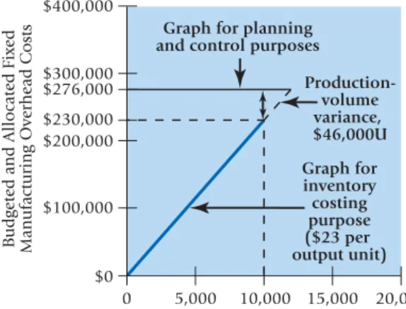
Exhibit 8-3 is a graphic presentation of the production-volume variance. Exhibit 8-3 shows that for planning and control purposes, fixed (manufacturing) overhead costs do not change in the 0- to 12,000-unit relevant range. Contrast this behavior of fixed costs with how these costs are depicted for the inventory costing purpose in Exhibit 8-3. Under generally accepted accounting principles, fixed (manufacturing) overhead costs are allo- cated as an inventoriable cost to the output units produced. Every output unit that Webb manufactures will increase the fixed overhead allocated to products by $23. That is, for purposes of allocating fixed overhead costs to jackets, these costs are viewed as ifthey had a variable-cost behavior pattern. As the graph in Exhibit 8-3 shows, the difference between the fixed overhead costs budgeted of $276,000 and the $230,000 of costs allo- cated is the $46,000 unfavorable production-volume variance.
Managers should always be careful to distinguish the true behavior of fixed costs from the manner in which fixed costs are assigned to products. In particular, while fixed costs are unitized and allocated for inventory costing purposes in a certain way, as described previously, managers should be wary of using the same unitized fixed overhead costs for planning and control purposes. When forecasting fixed costs, managers should concentrate on total lump-sum costs. Similarly, when managers are looking to assign costs for control purposes or identify the best way to use capacity resources that are fixed in the short run, we will see in Chapters 9 and Chapter 11 that the use of unitized fixed costs often leads to incorrect decisions.
Interpreting the Production-Volume Variance
Lump-sum fixed costs represent costs of acquiring capacity that do not decrease auto- matically if the resources needed turn out to be less than the resources acquired.
Sometimes costs are fixed for a specific time period for contractual reasons, such as an annual lease contract for a plant. At other times, costs are fixed because capacity has to be acquired or disposed of in fixed increments, or lumps. For example, suppose that acquiring a sewing machine gives Webb the ability to produce 1,000 jackets. Then, if it is not possible to buy or lease a fraction of a machine, Webb can add capacity only in incre- ments of 1,000 jackets. That is, Webb may choose capacity levels of 10,000; 11,000; or 12,000 jackets, but nothing in between.
Webb’s management would want to analyze why this overcapacity occurred. Is demand weak? Should Webb reevaluate its product and marketing strategies? Is there a quality problem? Or did Webb make a strategic mistake by acquiring too much capacity?
The causes of the $46,000 unfavorable production-volume variance will drive the actions Webb’s managers will take in response to this variance.
In contrast, a favorable production-volume variance indicates an overallocation of fixed overhead costs. That is, the overhead costs allocated to the actual output produced exceed the budgeted fixed overhead costs of $276,000. The favorable production-volume variance comprises the fixed costs recorded in excess of $276,000.
*
Budgeted and Allocated Fixed Manufacturing Overhead Costs
$400,000
$0 0
Output Units
20,000 15,000 10,000 5,000
$300,000
$276,000
$200,000
$230,000
$100,000
Graph for planning and control purposes
Production- volume variance,
$46,000U Graph for inventory costing purpose ($23 per output unit)
Behavior of Fixed Manufacturing Overhead Costs:
Budgeted for Planning and Control Purposes
and Allocated for Inventory Costing Purposes for Webb Company for April 2011
Exhibit 8-3
Be careful when drawing conclusions regarding a company’s decisions about capacity planning and usage from the type (that is, favorable, F, or unfavorable, U) or the magnitude associated with a production-volume variance. To interpret the $46,000 unfavorable vari- ance, Webb should consider why it sold only 10,000 jackets in April. Suppose a new com- petitor had gained market share by pricing below Webb’s selling price. To sell the budgeted 12,000 jackets, Webb might have had to reduce its own selling price on all 12,000 jackets.
Suppose it decided that selling 10,000 jackets at a higher price yielded higher operating income than selling 12,000 jackets at a lower price. The production-volume variance does not take into account such information. The failure of the production-volume variance to consider such information is why Webb should not interpret the $46,000 U amount as the total economic cost of selling 2,000 jackets fewer than the 12,000 jackets budgeted. If, how- ever, Webb’s managers anticipate they will not need capacity beyond 10,000 jackets, they may reduce the excess capacity, say, by canceling the lease on some of the machines.
Companies plan their plant capacity strategically on the basis of market information about how much capacity will be needed over some future time horizon. For 2011, Webb’s budgeted quantity of output is equal to the maximum capacity of the plant for that budget period. Actual demand (and quantity produced) turned out to be below the budgeted quantity of output, so Webb reports an unfavorable production-volume vari- ance for April 2011. However, it would be incorrect to conclude that Webb’s management made a poor planning decision regarding plant capacity. Demand for Webb’s jackets might be highly uncertain. Given this uncertainty and the cost of not having sufficient capacity to meet sudden demand surges (including lost contribution margins as well as reduced repeat business), Webb’s management may have made a wise choice in planning 2011 plant capacity. Of course, if demand is unlikely to pick up again, Webb’s managers may look to cancel the lease on some of the machines or to sublease the machines to other parties with the goal of reducing the unfavorable production-volume variance.
Managers must always explore the why of a variance before concluding that the label unfavorable or favorable necessarily indicates, respectively, poor or good management performance. Understanding the reasons for a variance also helps managers decide on future courses of action. Should Webb’s managers try to reduce capacity, increase sales, or do nothing? Based on their analysis of the situation, Webb’s managers decided to reduce some capacity but continued to maintain some excess capacity to accommodate unex- pected surges in demand. Chapter 9 and Chapter 13 examine these issues in more detail.
The Concepts in Action feature on page 280 highlights another example of managers using variances, and the reasons behind them, to help guide their decisions.
Next we describe the journal entries Webb would make to record fixed overhead costs using standard costing.
Journal Entries for Fixed Overhead Costs and Variances
We illustrate journal entries for fixed overhead costs for April 2011 using Fixed Overhead Control and the contra account Fixed Overhead Allocated (data from Exhibit 8-2).
1. Fixed Overhead Control 285,000
Salaries Payable, Accumulated Depreciation, and various other accounts 285,000 To record actual fixed overhead costs incurred.
2. Work-in-Process Control 230,000
Fixed Overhead Allocated 230,000
To record fixed overhead costs allocated
(0.40 machine-hour/unit 10,000 units $57.50/machine-hour). (The costs accumulated in Work-in-Process Control are transferred to Finished Goods Control when production is completed and to Cost of Goods Sold when the products are sold.)
*
*
3. Fixed Overhead Allocated 230,000
Fixed Overhead Spending Variance 9,000
Fixed Overhead Production-Volume Variance 46,000
Fixed Overhead Control 285,000
To record variances for the accounting period.
Overall, $285,000 of fixed overhead costs were incurred during April, but only $230,000 were allocated to jackets. The difference of $55,000 is precisely the underallocated fixed overhead costs that we introduced when studying normal costing in Chapter 4. The third entry illustrates how the fixed overhead spending variance of $9,000 and the fixed over- head production-volume variance of $46,000 together record this amount in a standard costing system.
At the end of the fiscal year, the fixed overhead spending variance is written off to cost of goods sold if it is immaterial in amount, or prorated among Work-in-Process Control, Finished Goods Control, and Cost of Goods Sold on the basis of the fixed overhead allo- cated to these accounts as described in Chapter 4, pages 117–122. Some companies com- bine the write-off and proration methods—that is, they write off the portion of the variance that is due to inefficiency and could have been avoided and prorate the portion of the variance that is unavoidable. Assume that the balance in the Fixed Overhead Spending Variance account as of April 2011 is also the balance at the end of 2011 and is immaterial in amount. The following journal entry records the write-off to Cost of Goods Sold.
Cost of Goods Sold 9,000
Fixed Overhead Spending Variance 9,000
We now consider the production-volume variance. Assume that the balance in Fixed Overhead Production-Volume Variance as of April 2011 is also the balance at the end of 2011. Also assume that some of the jackets manufactured during 2011 are in work-in- process and finished goods inventory at the end of the year. Many management account- ants make a strong argument for writing off to Cost of Goods Sold and not prorating an unfavorable production-volume variance. Proponents of this argument contend that the unfavorable production-volume variance of $46,000 measures the cost of resources expended for 2,000 jackets that were not produced ($23 per jacket 2,000 jackets =
$46,000). Prorating these costs would inappropriately allocate fixed overhead costs incurred for the 2,000 jackets that were not produced to the jackets that were produced.
The jackets produced already bear their representative share of fixed overhead costs of
$23 per jacket. Therefore, this argument favors charging the unfavorable production- volume variance against the year’s revenues so that fixed costs of unused capacity are not carried in work-in-process inventory and finished goods inventory.
There is, however, an alternative view. This view regards the denominator level cho- sen as a “soft” rather than a “hard” measure of the fixed resources required and needed to produce each jacket. Suppose that either because of the design of the jacket or the functioning of the machines, it took more machine-hours than previously thought to manufacture each jacket. Consequently, Webb could make only 10,000 jackets rather than the planned 12,000 in April. In this case, the $276,000 of budgeted fixed overhead costs support the production of the 10,000 jackets manufactured. Under this reasoning, prorating the fixed overhead production-volume variance would appropriately spread fixed overhead costs among Work-in-Process Control, Finished Goods Control, and Cost of Goods Sold.
What about a favorable production-volume variance? Suppose Webb manufactured 13,800 jackets in April 2011.
Because actual production exceeded the planned capacity level, clearly the fixed overhead costs of $276,000 supported production of, and so should be allocated to, all 13,800 jackets.
Prorating the favorable production-volume variance achieves this outcome and reduces the amounts in Work-in-Process Control, Finished Goods Control, and Cost of Goods Sold.
Proration is also the more conservative approach in the sense that it results in a lower
= $276,000 - $317,400 = $41,400 F
= $276,000 - ($23 per jacket * 13,800 jackets) Production-volume variance =
Budgeted fixed overhead
-
Fixed overhead allocated using budgeted cost per output unit overhead
allowed for actual output produced
*
operating income than if the entire favorable production-volume variance were credited to Cost of Goods Sold.
One more point is relevant to the discussion of whether to prorate the production- volume variance or to write it off to cost of goods sold. If variances are always writ- ten off to cost of goods sold, a company could set its standards to either increase (for financial reporting purposes) or decrease (for tax purposes) operating income. In other words, always writing off variances invites gaming behavior. For example, Webb could generate a favorable (unfavorable) production-volume variance by set- ting the denominator level used to allocate fixed overhead costs low (high) and thereby increase (decrease) operating income. The proration method has the effect of approximating the allocation of fixed costs based on actual costs and actual output so it is not susceptible to the manipulation of operating income via the choice of the denominator level.
There is no clear-cut or preferred approach for closing out the production-volume variance. The appropriate accounting procedure is a matter of judgment and depends on the circumstances of each case. Variations of the proration method may be desir- able. For example, a company may choose to write off a portion of the production- volume variance and prorate the rest. The goal is to write off that part of the production-volume variance that represents the cost of capacity not used to support the production of output during the period. The rest of the production-volume vari- ance is prorated to Work-in-Process Control, Finished Goods Control, and Cost of Goods Sold.
If Webb were to write off the production-volume variance to cost of goods sold, it would make the following journal entry.
Decision Point
What variances can be calculated for fixed overhead costs?
Learning Objective 5
Show how the 4-variance analysis approach reconciles the actual overhead incurred with the overhead amounts allocated during the period . . . the 4-variance analysis approach identifies spending and efficiency variances for variable overhead costs and spending and production-volume variances for fixed overhead costs
Cost of Goods Sold 46,000
Fixed Overhead Production-Volume Variance 46,000
Integrated Analysis of Overhead Cost Variances
As our discussion indicates, the variance calculations for variable overhead and fixed overhead differ:
䊏 Variable overhead has no production-volume variance.
䊏 Fixed overhead has no efficiency variance.
Exhibit 8-4 presents an integrated summary of the variable overhead variances and the fixed overhead variances computed using standard costs for April 2011. Panel A shows the variances for variable overhead, while Panel B contains the fixed overhead variances.
As you study Exhibit 8-4, note how the columns in Panels A and B are aligned to measure the different variances. In both Panels A and B,
䊏 the difference between columns 1 and 2 measures the spending variance.
䊏 the difference between columns 2 and 3 measures the efficiency variance (if applicable).
䊏 the difference between columns 3 and 4 measures the production-volume variance (if applicable).
Panel A contains an efficiency variance; Panel B has no efficiency variance for fixed over- head. As discussed earlier, a lump-sum amount of fixed costs will be unaffected by the degree of operating efficiency in a given budget period.
Panel A does not have a production-volume variance, because the amount of variable overhead allocated is always the same as the flexible-budget amount. Variable costs never have any unused capacity. When production and sales decline from 12,000 jackets to 10,000 jackets, budgeted variable overhead costs proportionately decline. Fixed costs are different. Panel B has a production-volume variance (see Exhibit 8-3) because Webb had to acquire the fixed manufacturing overhead resources it had committed to when it planned production of 12,000 jackets, even though it produced only 10,000 jackets and did not use some of its capacity.
4-Variance Analysis
When all of the overhead variances are presented together as in Exhibit 8-4, we refer to it as a 4-variance analysis:
PANEL A: Variable (Manufacturing) Overhead
Flexible Budget: Allocated:
Actual Costs Budgeted Input Quantity Budgeted Input Quantity
Incurred: Allowed for Allowed for
Actual Input Quantity Actual Input Quantity Actual Output Actual Output
Actual Rate Budgeted Rate Budgeted Rate Budgeted Rate
(1) (2) (3) (4)
(0.40 hrs./unit 10,000 units $30/hr.) (0.40 hrs./unit 10,000 units $30/hr.) (4,500 hrs. (4,500 $29/hr.) hrs. $30/hr.) (4,000 hrs. $30/hr.) (4,000 hrs. $30/hr.)
$130,500 $135,000 $120,000 $120,000
$4,500 F $15,000 U
Spending variance Efficiency variance Never a variance
$10,500 U
Flexible-budget variance Never a variance
$10,500 U
Underallocated variable overhead (Total variable overhead variance) PANEL B: Fixed (Manufacturing) Overhead
Flexible Budget:
Same Budgeted
Same Budgeted Lump Sum Allocated:
Lump Sum (as in Static Budgeted Input Quantity
(as in Static Budget) Budget) Allowed for
Actual Costs Regardless of Regardless of Actual Output
Incurred Output Level Output Level Budgeted Rate
(1) (2) (3) (4)
(4,000 hrs. $57.50/hr.)
$285,000 $276,000 $276,000 $230,000
$9,000 U $46,000 U
Spending variance Never a variance Production-volume variance
$9,000 U $46,000 U
Flexible-budget variance Production-volume variance
$55,000 U
Underallocated fixed overhead (Total fixed overhead variance)
aF = favorable effect on operating income; U = unfavorable effect on operating income.
(0.40 hrs./unit 10,000 units $57.50/hr.) Exhibit 8-4 Columnar Presentation of Integrated Variance Analysis: Webb Company for April 2011a
4-Variance Analysis
Spending Variance Efficiency Variance Production-Volume Variance
Variable overhead $4,500 F $15,000 U Never a variance
Fixed overhead $9,000 U Never a variance $46,000 U