a perturbation procedure for nonlinear oscillations

(THE DYNAMICS OF TWO OSCILLATORS WITH WEAK NONLINEAR COUPLING)

Thesis by

Howard Arthur Kabakow

In Partial Fulfillment of the Requirements

For the Degree of Doctor of Philosophy

California Institute of Technology Pasadena, California

1969

(Submitted November 25, 1968)

ACKNOWLEDGMENTS

The author acknowledges with deep respect and gratitude the guidance of his research advisor, Professor Julian D. Cole, whose suggestions led to the choice of problems studied in this thesis and who gave freely of his time to help with the difficulties encountered in

resolving them.

He also wishes to express his appreciation to Professor Richard P. Feynman for his interest in this work and for a number of stimulating discussions which contributed materially to its progress;

to Mrs. Vivian Davies for her careful and accurate typing of the rough and final drafts; to Mr. Richard Casten for valuable assistance and suggestions in preparing the manuscript; to the National Science Foundation which contributed financial support through NSF Grant GP 7978; and to the California Institute of Technology for various scholarships, fellowships and assistantships.

Finally, the author wishes to thank his wife Lynn for her continuing encouragement and understanding during the course of this work.

ABSTRACT

This thesis considers in detail the dynamics of two oscillators with weak nonlinear coupling. There are three classes of such problems:

non-resonant, where the Poincare procedure is valid to the order considered; weakly resonant, where the Poincare procedure breaks down because small divisors appear (but do not affect the 0(1) term) and strongly resonant, where small divisors appear and lead to 0(1) corrections. A perturbation method based on Cole's two-timing pro- cedure is introduced. It avoids the small divisor problem in a straight- forward manner, gives accurate answers which are valid for long times, and appears capable of handling all three types of problems with no

change in the basic approach.

One example of each type 1s studied with the aid of this procedure: for the nonresonant case the answer is equivalent to the Poincare result; for the weakly resonant case the analytic form of the answer is found to depend (smoothly) on the difference between the initial energies of the two oscillators; for the strongly resonant case we find that the amplitudes of the two oscillators vary slowly with time as elliptic functions of E t, where E is the (small) coupling parameter.

Our results suggest that, as one might expect, the dynamical behavior of such systems varies smoothly with changes in the ratio of the fundamental frequencies of the two oscillators. Thus the pathological behavior of Whittaker's adelphic integrals as the frequency ratio is

varied appears to be due to the fact that Whittaker ignored the small divisor problem. The energy sharing properties of these systems appear to depend strongly on the initial conditions, so that the systems

are not ergodic.

The perturbation procedure appears to be applicable to a wide variety of other problems in addition to those considered here.

TABLE OF CONTENTS

PART TITLE

Introduction I

II

III

IV

v

VI

Discussion of Previous Literature on Coupled Oscillators The "N -timing" Perturbation Procedure

A. The Necessity for Uniform Validity and the Small Divisor Problem

B. The Method of N- timing A Non-Resonant Example

A. Solution of the Equations of Motion by N-timing B. Comparison with Computer Experiments

A "Weakly Resonant" Example A Strongly Resonant Example Summary and Conclusions

APPENDICES

Appendix A The Significance of Ergodicity in Statistical

PAGE 1 4 10

10 14 20

21 36

40 61 72.

Mechanics 78

Appendix B Algebraic Details of and Comments on Chapter IV 83

REFERENCES 89

Introduction

Problems involving systems of oscillators with weak nonlinear (polynomial) coupling have long been of interest in connection with the ergodic problem of statistical mechanics (see Appendix A) and as simple models of nonlinear interactions. In the present work we will consider in detail problems of two such oscillators, with our objective being to determine the long- term behavior of the gross properties and the detailed dynamics of such systems.

One question of particular interest in connection with the ergodic problem is whether a particular coupled system permits signif-

*

icant energy to be exchanged among the degrees of freedom. Since

energy sharing is a necessary (but not sufficient) condition for ergodicity and presumably easier to establish than ergodicity, it can be used as a preliminary test- no energy sharing implies no ergodicity. Energy sharing is also of interest with respect to the question of equipartion- is a simple nonlinear coupling sufficient to insure that the time averaged energies of the degrees of freedom will be approximately the same?

Of course the direct relevance of these questions and indeed of these systems to statistical mechanics is describable only in terms of the thermodynamic limit, where the number of degrees of freedom of

>:'we will use the term degrees of freedom with reference to coordinate systems in which the subsystems remain weakly coupled, e.g. particle coordinates, rnode coordinates.

the system goes to infinity, but we suggest that it will be easier to

understand large systems if we understand clearly the behavior of small ones. At the same time, we hope that the information obtained by our examination of small systems will shed some light on the behavior of large ones.

In addition to being model systems for statistical mechanical problems, the examples we will study here are directly relevant to understanding the long- time behavior of simple nonlinear systems.

Perturbation methods have frequently been applied to such systems with varying degrees of success; however, a significant question has been left open, presumably because the answer is not obtainable by most usual approaches. This difficulty has been mentioned frequently in the literature, and is generally referred to as the small divisor problem.

The first chapter of this thesis describes some interesting results of the work of previous investigators of systems of coupled oscillators. Chapter II discusses the small divisor problem, points out certain of the other difficulties inherent in applying various standard perturbation procedures to coupled oscillator systems, and introduces and describes ¹¹N-timing, ¹¹ the approach which is to be used in the present work. In Chapter III we work a non- resonant problem which can be done equally well by other methods (e.g. Poincare, Wigner-Brillouin), and in Chapter IV we work a problem which explicitly demonstrates the ability of N- timing to remove small divisors. Chapter V will present our solution of a ¹¹ strongly resonant¹¹ problem, where the energy-

sharing can be 0(1). Chapter VI discusses our results and their relevance to some of the questions raised in the foregoing paragraphs.

Appendix A examines the importance of ergodicity in statistical mechanics, and Appendix B presents some algebraic details omitted from the text.

Chapter I

Discussion of Previous Literature on Coupled Oscillators.

E. T. Whittaker and Henri Poincare were prominent among early workers contributing to the theory of nonlinear oscillations.

*

Poincare (1893) devised a useful and ingenious perturbation procedure which we shall discuss in Chapter II. Whittaker (1916) studied in detail

the problem of two oscillators with weak nonlinear coupling, and found that for such a system one can always, at least formally, construct a constant of the motion

cp ( x, ^dx

.£y

dt ' y' dt '

different from the total· energy and analytic in the dynamical variables

**

and E.

To construct these constants, which he called ¹¹adelphic integrals, ¹¹ Whittaker found it necessary to distinguish three cases depending on the frequencies w₁ and w₂ of the two oscillators and the form of the coupling:

_C_a_s_e_l....:.·) __ w._.L₁ :.../_w_,₂.___is irrational;

>!<A name followed by a date is used to refer to an entry in the list of references.

>:<*Throughout this thesis, E will generally be a small dimensionless

parameter of the order of the coupling term in the Hamiltonian; i.e. - we are considering systems with

Case 2) w₁ /wz is rational, and the system is "weakly resonant";

Case 3) rational, and the system is "strongly resonant."

Here we have used our own terminology as to the types of resonance in order to avoid reference to and transformation to action angle variables of a specific problem. We will discuss weak and strong resonance in more detail later; for now it will be sufficient to state that, phenomena-

logically speaking in terms of applying the Poincare procedure to the problem in question, by weak resonance we mean that there are no O(lt additive corrections to the 0(1) term of the solution arising from higher iterations - by strong resonance we mean that there are such corrections.

Each of the three cases distinguished above leads, in Whittaker's formalism, to a different analytic form for the adelphic integral.

Whittaker's work raises two questions: do the series defining the adelphic integrals converge, and if they do what is implied by the fact that the series change form drastic ally over arbitrarily small changes in the frequency ratio? With regard to the first question, we suspect that one can think of examples where Whittaker's formalism will lead to apparently divergent adelphic integrals. As to the second, we suggest that if Whittaker attempted to eliminate small divisors, the series for an irrational frequency ratio would resemble that for a neigh- boring rational ratio, since we expect a much smoother dependence on the frequency ratio than Whittaker's results appear to indicate. These

*rn this thesis ffJ (E, t) = 0 ( l)J(E)) will mean

;~:~t)

^and

PJ7;~)

both remain bounded as ^E tends to O(t fixed) for "almost all" t (except possibly for a set of measure zero of t¹ s).

questions are still open, but even if the adelphic integrals diverge it appears likely that one can find functions which are constant to some

p p+l

order, say E , then variable only by an amount of order E

More recently, several authors have considered problems involving two or more oscillators with the aid of mechanical computation as well as analytic techniques, the former giving these authors, in a sense, experimental results to check their theoretical solutions. Among the significant contributions of this type are those of Fermi, Pasta and Ulam (1955), Ford and Waters (1963) and E. A. Jackson (l963a, l963b).

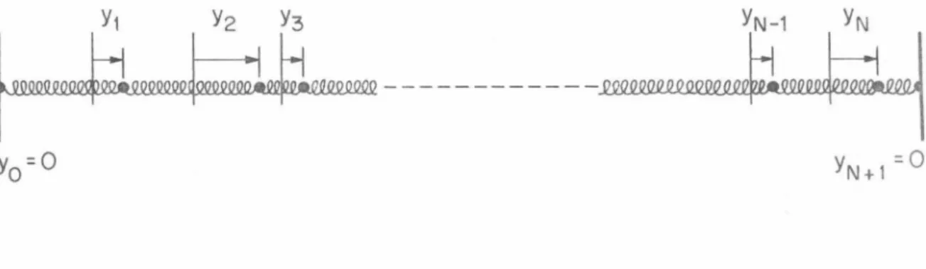
FPU performed computer studies of a one dimensional chain of identical particles connected by identical, weakly nonlinear springs. The

configuration of their system is represented in Fig. l.

Y1 Y2 Y3 YN-1 YN

~og_ooooQJ1Jj,.,,.~,,;;iJ;!W>oo<>Ql1 - - - -- -- - -- - -.Q.Qli~ru~?W1Qfl.e.-£llll!JJi.~~llee!fl.1

y =0

0

Fig. l. Configuration of FPU System

yk is the displacement of the kth particle from its equilibrium position.

The potential energy of the spring connecting the kth particle to the k + l s t is (in dimensionless coordinates)

2 3

v

k,k+l =

i

(yk+l- yk) +

3 (

^{yk+l- yk)}

Thus the FPU Hamiltonian is · (still in dimensionless coordinates)

= z

1

N k=l

L:

(1)

Transforming to mode coordinates (based on the linear normal modes), the Hamiltonian becomes:

with

w q = 2 sin ⁹71'

2(N+l)

( 2)

We will refer to systems with Hamiltonians of the form (2) as ¹¹FPU- type systems. ¹¹

Contrary to their expectations, FPU found that their system was not ergodic since energy was not shared uniformly among the modes - when the system was started with all the energy in the first mode only the first few modes became appreciably excited. This interesting result was the starting point for several subsequent studies of coupled oscil- lators, prominent among which - were the work of Ford and Waters (1963)

and of Jackson (1963a), (1963.b).

Ford and Waters used the Wigner-Brillouin perturbation theory (which is similar to Poincare's method) and mechanical compu- kation to study conservative systems of from two to fifteen oscillators with weak cubic coupling in the Hamiltonian. Their theoretical work and

supporting machine computations showed that such systems can exhibit

significant (i.e., 0(1) ) energy sharing among all the modes only if the

I

fundamental frequencies ~ are respectively near certain integral multiples of some basic frequency. Furthermore, they found that even when the frequencies are in the right ratios there exist certain sets of initial conditions which do not permit significant energy exchange. This being the case, they concluded that nonlinear systems of the type they

studied are not ergodic.

They also examined the behavior of a particular five-oscillator system which had the appropriate frequencies and initial conditions for energy sharing and found that in such a system, the amount of time a single oscillator (mode) spends with energy between E and E

+

oE is roughly proportional to exp (-E/E_{0 ),} where E₀ is the total energy in the system divided by the number of oscillators. Thus, the remaining oscillators form a "heat bath" for the one under consideration and the canonical distribution appears without benefit of ergodicity.

Ford and Waters' analytic results for non- resonant systems were in agreement with their mechanical computations and the results of

our N- timing procedure. However, the Wigner- Brillouin procedure, like the Poincare technique, is inherently incapable of handling strongly resonant systems, since terms of 0(1) will generally appear in an

infinite number of iterations. As we shall see later, such behavior means we are putting the answer in the wrong analytic form; the slow variation of the solution is not necessarily a frequency shift, butpossibly a different function of the slow time variables.

Jackson used a modified Wigner-Brillouin procedure to study FPU- type systems with moderate values of the coupling parameter (e.g.

.1/4, 1

/z,

^3/_{4 ).} He found that the sizes of the frequency shifts due to the nonlinear coupling were significant in determining the amount of energy exchanged among the modes and the recurrence time of the initial distri- bution of energy, and his theoretical results for these quantities agreed

rather well with his machine calculations. Like Ford and Waters, Jackson pointed out that the energy sharing behavior of such systems depends strongly on initial conditions, and an F:PU- type ensemble starting with all its energy in the low modes will tend to keep most of its energy in the low modes. Finally he pointed out that small changes in the initial conditions will not cause substantial changes in the gross properties of the solution.

Jackson's perturbation approach, while effective in predicting the gross behavior of the systems he studied, is somewhat less usefulin giving explicit solutions to the dynamical problems. One reason is that his coupling constants are too large to permit the terms of his series to

decrease in size rapidly, but more important, the same observations apply to his rriethod as to Ford's method described above; the Wigner- Brillouin approach breaks down near resonances, and as an FPU system tends to a large number of degrees of freedom, the frequencies of the lower modes approach the resonant ratios. Thus Jackson's method is not useful for studying the detailed dynamics of large systems. More- over, for certain classes of initial conditions higher order resonances are possible for systems of as few as two oscillators, even with in- commensurable frequencies, and neither does Jackson's method apply

to this problem.

Chapter II

The "N -timing" Perturbation Procedure

A. The Necessity for Uniform Validity and the Small Divisor Problem.

The problems to be studied in the present work are members of a class of problems involving small forces which are active for a long time. The basic systems we shall consider are derivable from Hamiltonians of the form (in dimensionless units):

with corresponding equations of motion

and·

0< IEI<<l, ~ ~

^{0 (1) '}

~ ~

^{0 (1)}

~ The initial conditions to be satisfied are

= b k

(1)

gk is a polynomial in the ~· s and at first we are thinking about the d~

limit ^{E -} 0, t fixed. The dynamic variables ~ and

<ft

will usually correspond to the amplitudes and time rates of change of the amplitudes of the normal modes of oscillation of a system which is linear if E

=

^0.

We assume that we know by physical or other considerations that the dynamical variables ~ and ~ d~ are bounded.

The solutions of such systems are for times t ~ 0(1)

equivalent to 0(1) to the solutions of the un~oupled equations; i.e., to

the solutions of equations (l) with E

=

0. As time passes, however, the weak forces will cause the exact solutions of equations (l) to driftaway or bifurcate from those of the uncoupled equations, and eventually the error engendered in using the initially valid solutions in place of the exact solutions·will be 0(1). Alternatively, if we look at the solution of system (l) in the time interval T

<

t

<

T

+ o

^{T, where T ~ O(l/E2 ) and}

or=

^{0(1), to 0(1)} the motion will look like the solution of the uncoupled equations with initial conditions different from equations (2) (but of course located on the same energy shell), Thus, to 0(1) the solutions of

equations (l) look like those of the uncoupled equations with slowly varying initial conditions.

A consequent difficulty often encountered in applying pertur- bation procedures to such problems is that the resulting solutions are only valid initially - after a certain initial time the magnitude of the

.

higher correction terms becomes equivalent to or larger than that of the lowest order terms, and consequently an infinite number of terms is needed to adequately describe the answer. The classical procedure for eliminating this difficulty, and the one which has generally been applied to the kind of systems we are studying here,is the well-known Poincare technique, which seeks to allow for the nonlinearity by introducing small shifts in the fundamental frequencies of the oscillators.

The Poincare procedure works effectively if the frequencies are ¹¹ sufficiently incommensurable, ¹¹ and in many cases for a certain delimited span of time when they are commensurable. However, trig- onometric terms of various combination frequencies appear on the right hand sides of all iterations subsequent to the first, and if one of these

combination frequencies is ¹¹ sufficiently clos e¹¹ to the fundamental frequency of the equation in which it appears, the corresponding small resonance denominator can push the amplitude of the resulting term in the solution to a larger order than it was originally thought to be. Further- more, once such a small divisor appears, it frequently appears in

successively higher powers in subsequent interactions, raising a term from each of these iterations to the increased order of the term where the small divisor first appeared. The appearance of such terms in the solution thus tends to break down the uniform validity of the solution and raise questions about the convergence of the expansion.

A related situation is the case where the frequencies are commensurable but not in a ratio which will cause strong resonance (i.e., 0(1) corrections to the solution due to small divisors). In this case one can obtain combination frequencies whose 0(1) terms vanish identically. However, the small corrections to the combination frequen- cies usually do not vanish, so if an appropriately modified Poincare scheme is used, this situation reduces to the usual small divisor

problem. In the work that follows, we shall call cases where no small divisor appears to the order considered non-resonant, and where they do appear, weakly resonant. We suggest, however, that there is not

necessarily a sharp dichotomy between the two cases - the small ':<

divisors in the latter case may just take longer to appear.

::!c

It is not difficult to see how small divisors can appear at some point in the Poincare expansion for any given pair of frequencies w₁ , w₂ • Given any pair of incommensurable numbers w₁ and w₂ and any 6

>

0, there

exist infinitely many pairs of (positive) integers n, m such that

jnw_{2 -} mw₁ j

<

6. However, for polynomial coupling, the larger the values

of n and m, the further out in the series the corresponding combination frequency will appear. It does not seem apriori obvious (without actually

In some cases, near particular frequency ratios which corres- pond to the form of the nonlinearity, one finds that small denominators occur in the initial iterations of the Poincare scheme and raise the corresponding terms to 0(1), thus causing 0(1) corrections to the answer. In such cases, to which we will refer as ¹¹ strongly resonant, ¹¹ the Poincare procedure is useless (except for establishing that the strong resonance exists) and one usually attempts to establish the 0(1) solution by other means, most of which involve certain transformations of the original equations.

Several sophistic a ted techniques have been developed to deal with the difficulties mentioned in the foregoing paragraphs, including Krylov and Bogoliubov¹ s method of averaging (Bogoliubov and

Mitropolsky, 1961), Struble's general asymptotic method (Struble 1962) and Cole's two- timing procedure (Cole 1968). This chapter will intro- duce N-timing, which is an extension of two-timing.

In the work that will follow, we will find that the small divisor problem can be eliminated with the assistance of a sufficiently flexible perturbation procedure. N-timing appears to be such a procedure, and it will be used to study a non-resonant example which is also tractable by Poincare's method, as well as weakly and strongly resonant examples

(continued from preceding page)

calculating the expansion) how to tell whether or not a particular com- bination frequency (nwz - mw_{1 )} will appear but we can easily provide a bound for the order of the term in which a small divisor will first appear by the following procedure. Suppose H¹ (the perturbing Hamiltonian) is a polynomial of order k. Let the term where a small divisor first appears in the Poincare expansion of the solution of the equations of motion resulting from the perturbed Hamiltonian

Ho

+ EH¹ be 0(E1).

Let (N, M) be the pair of integers satisfying

I

^{nwz - mw}1

I =

^{O{E) and}

having the smallest value ln+ml of all such pairs. Then 1 ~(smallest integer ~(N+M-1/k-2)-1 ).

which are not.

B. The Method of N-timing.

The simplest perturbation procedure we can apply to a problem like (1) is a limit-process expansion wherein we let

(2)

substitute (2) for ~ in (1), and set the coefficient of each Ep in each of the N resulting equations separately equal to zero. This yields a system of N equations of each order in E which in turn leads to a sequence of problems which can be solved in series (because of the limit process E - 0).

0(1)

O(E)

The equations of orders 1 and E dZ ~o)

+

^w z x. (o)

=

⁰

dtZ k · K

are:

dZ x(1)

---:--:::-'k~

+

z x. (1) = _Qg_ (x (o) x. (o) x (o))

dtZ wk K

a

¹ ' ••• ' K ' ••• ' N

~

(3)

(4)

This system can be solved by first solving (3), then replacing the

~o),s

in the right-hand side of (4) with the corresponding solutions of equations (3). However, one will generally find terms proportional to t appearing in the solutions for

~

¹

) o~ ~z).

Moreover, once such terms start to appear, one will find a higher power of t in each succeeding term, so that although these solutions may be valid to 0(1) for t = 0(1), it is clear that the exact solutions cannot be represented accurately to 0(1) by a finite number of terms for t ~ 0( ¹/E) or 0( ¹/c-EZ) (depending on

whether the t first appears in the O(E) or O(EZ) term of the expression for

xJ·

This difficulty is clearly connected with the difficulty described in the introduction above, the fact that the solutions of (1) to 0(1)

resemble the solutions of the uncoupled equations with slowly varying initial conditions. The solutions obtained by this simple limit process

expansion always have as an 0(1) term the solutions of the uncoupled equations with constant initial conditions. The divergent terms are

telling us that we must allow for some change in the form of the 0(1) term due to the presence of the weak forces.

The classical procedure for eliminating this difficulty was developed by Poincare (1893). He suggested that the effect of the weak forces is to cause a slight shift in the frequencies wk. Thus he proposed that one replace the wk¹ s by

( 5)

where the

w~i)

¹ s and Ok are constants to be determined. Then equation (l) becomes

(6)

where 0 2 - w²

=

^O(E). Substituting expansions of the form (2) for the k k

~ in equations (5) and setting the coefficients of each Ep in each of the resulting equations equal to zero, we obtain a system of N equations of each order in E. The equations of order l and E are now:

0(1)

dz ~o)

dtZ

+ Ok_ ~o)

^{= 0 (7)}

O(E) (8)

Solving equation (7) we obtain:

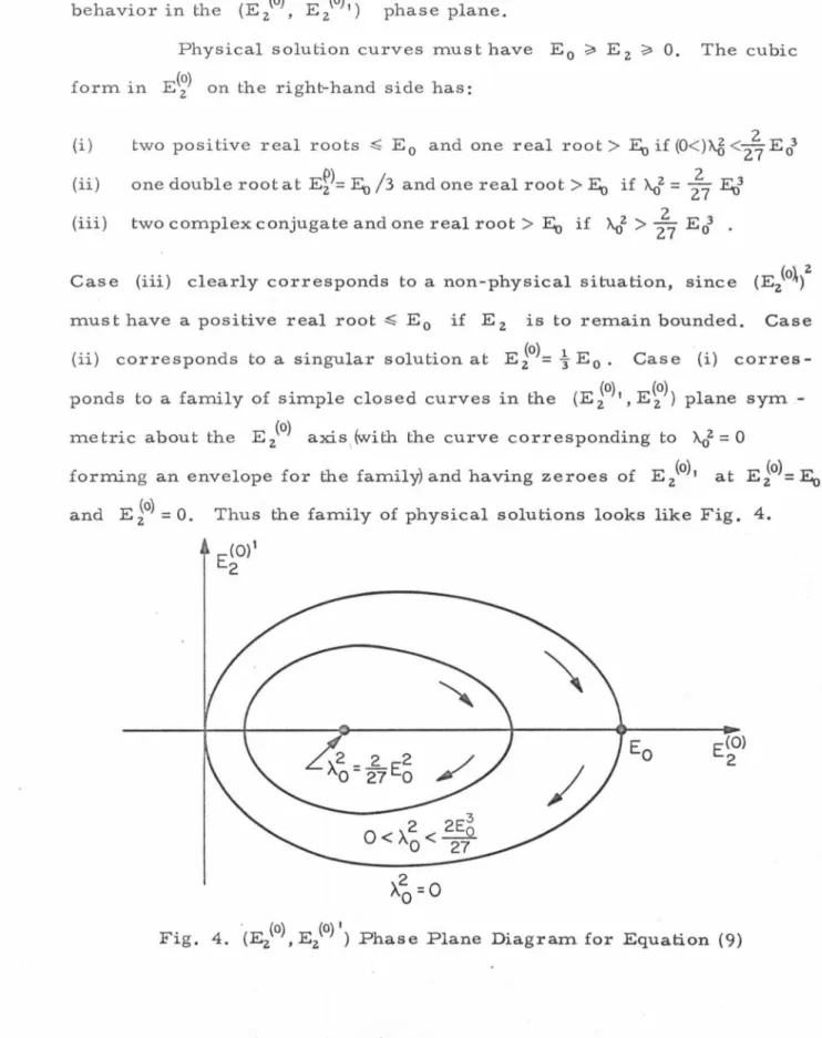
(9)

Replacing each

~o)

by its solution on the right hand side of (8) with its value (9), we obtain a set of linear oscillators with forcing terms whose frequencies are appropriate combinations of the nk. The term

2w~O) w~l) ~o)

has a frequency identical to the fundamental, nk. This and other of the driving terms which have frequency nk (e.g., a term like xZ

1 ^~) are called secular terms and will lead to terms of the form t sin(Okt -

cp~o)

in the expression for x_{1 ,} unless the sum of the co- efficients of such driving terms vanishes. Since a useful perturbation theory requires that the terms be uniformly ordered - i.e., that the terms of O(E) remain smaller than the terms of 0(1), etc. - and we are free to choose the

w~

¹

)

¹

s

to suit our convenience, we choose the

w~

¹

)

¹

s

such that the secular terms vanish. We then choose the

w~z.),s

by repeating this procedure with the 0(E2 ) equations and so forth.

The Poincare procedure is quite useful for studying systems that reduce to a single oscillator. Unfortunately, it will generally break down in some order when N ~ 2. For example, suppose N

=

^{2, w}1

=

^l,

wz.

=

2, and a term x₁² x₂ appears in the Hamiltonian. This leads to a term

i

^{a1(o) z cos (2 n1 t-} 2cp1{o) ) in the right-hand side of the equation for

x}

^1). This is not a secular term, so it leads to a term like cos { _{2 n 1} t - _2cp1 (0) }

nz _

402

2 1

· th · f (¹⁾ How' ever, ,..., 2 + (l)+

~n e expres ^s~on or x₂ • u 2

=

^{E w}₂ ^{• • •}

~

= l + E w1 (

1) + • • . s 0 that O.f - 4 _f21Z = E ( 4w2 (

1)-

8~

(¹) ) + 0 (E 2), and

and thus one of the terms supposedly of O(E) makes an 0(1) contribution to the

expression for

:xz.

Furthermore, subsequent higher order terms may also make contributions in 0(1) and the Poincare theory thus becomes useless for this case.

In cases where such a breakdown does not occur in the O(E) solution it may still occur later. For the case N

=

2, it is easy to see how this can happen if w₁ and w₂ are commensurable. Of course, if

they are incommensurable, it may also occur if we have nw_{1 -} mw₂

=

O(E) and one of the iterations, say O(E ) leads to a r term with frequency

This implies a term contributing to O(E r-1 ) and the further

validity of the procedure becomes doubtful. The solution is probably valid to O(E r-2 ) but questionable thereafter; thus we can follow the

oscillator for a time ¹

/E

^r-2 but since we are not sure of the frequencies wk(r-¹), we lose track of it for larger times. This is the famous problem of small divisors.

The N -timing procedure which we shall now introduce and describe avoids the difficulties described above by anticipating that the slow changes with time of the solutions of equations (1) may be more complicated than simple frequency shifts.

To employ the N-timing procedure we assume that the slow variation of the solutions of equations (1) can be represented by formally considering the solutions to be functions of a sequence of related but (formally) independent variables;

tv,

t1 , ••• , tk, ... , where the new

k >l<

variables are related to t by the relations ~ = E t. We then use expansions for the ~ of the form:

~(t) (o) (1) 2 (2)

=

^{xk (}

l:a ,

t1 , • . • , t q , ... ) + E ~ ( t₀ , t1 , .•• ) +E ~

(tv ,

t_{1 ,} ^{••• ) (} 10)

.,_

-~A more general plan would have ~

=

cpk(E) t, where the cpk(E) form an asymptotic sequence.

Derivatives with respect to t now become:

(11)

so that

(12)

and

d2~

We now replace ~(t) and

"dt2"

in equations (1) by their correspond- ing expansions, equations (10) and (12). Setting the coefficients of each power of E in each equation separately equal to zero we obtain a system of N equations of each order in E . The equations of 0(1) and O(E) are respectively,

azx(o)

k ₂ (o)

otJ

^{+ wk} ~

=

⁰

0(1) (13)

O(E) (o) (o) (o)

xz , ... ·~, ···~) ⁽¹⁴⁾

The fundamental principle of expansion is that each term appearing in a solution of a particular order must be uniformly of that order. This excludes terms increasing like t, as well as terms with coefficients such as

1/E

that raise a term to a larger>:< order. Such terms must be eliminated by choosing the proper dependence of larger order terms on the slow time variables, in the spirit of the procedure for removing

>:<Throughout, to avoid ambiguity, larger order will mean larger magnitude - i.e., 0(1) is larger order than O(E).

secular terms 1n the Poincare technique.

TheN-timing method is capable of handling all problems which can be done by the Poincare technique, but more important, it provides a method for solving problems with resonant or near resonant frequencies where the Poincare technique is manifestly inapplicable.

N- timing also has the aesthetic feature that with no modification it is applicable to a variety of problems including both resonant and non- resonant systems like equations (l). In the present work we shall apply N -timing to three examples, one where no resonance appears to the order considered, and two others where resonances become significant early and lead to interesting consequences. ·

For a more detailed discussion and examples of the two-

timing procedure, of which N-timing is an extension, refer to Cole (1968, Chapter III), and Kevorkian (1966). Unknown to the present author at the time this work was done similar expansions were proposed by Sandri (1966) previous to and Lick (1968) simultaneously with the present work.

However, neither author applied the procedure to problems of the type we are considering. Lick applied it to singular problems and some partial differential equations from fluid mechanics and Sandri to some

*

quantum mechanical examples.

:>',<

It should also be noted that Eckstein, Shi and Kevorkian (1964) studied an orbital mechanics problem which required the use of three time variables for solution. However, it appears that the third variable was used because the problem involved matching of solutions in two regions which required different slow variables. Therefore the approach used

does not seem to be directly comparable with N-timing.

Chapter III

A Non-resonant Example

The first example we will consider is a non- resonant case, a two- oscillator FPU system, where to the order considered the Poincare procedure will give the same result as N-timing.

The system of equations to be solved is derived from the

*

Hamiltonian

(1) For convenience, the equations will be solved in normal mode coordinates x, y where:

x=zl+zz

.[2

is the amplitude of the symmetric mode and

y

=

Zz- zl is the amplitude of the antisymmetric mode .

.[2

Applying transformation (2) to the Hamiltonian (1) and letting:

t

=

^{3 t}

.fi.

we obtain:

H(x,y,:k,y)

* ^{£ =}

_- ^df(t) _dt

The equations of motion are thus:

d2x dtZ

+

x = 2Exy

(2)

(3)

(4)

(5a)

y(O)

=

^c

(~)\ =

^d

t=O

(5b)

A. Solution of the Equations of Motion by N-timing.

We shall apply the N- timing procedure to equations (5). Let

where

so that

00 k

x ( t)

= 2:

^€ ~ ( t_{0 ,} t _{1 ,} ••• )

k=O

00

y(t) =

2:

€1 y1(to,ti, ... ) 1=0

The operator

d ⁰⁰ k 8 dt

=I:

_k=O ^{€ 8t..} _~k

d2 00 k { k 82 } dtZ =

L

^€

L

^8t

8~

k=O p=O p -p

(6a)

(6b)

(7)

(8)

Using expressions (6a) and (6b) for x and y and equation

d² k

(8) for dtZ in equations (5) and equating the coefficient of € in each of the resulting equations to zero, we obtain a double sequence of

equations of decreasing order in €. The equations we shall need are:

82xo

+

xo = 0

8toz (9a)

0(1)

82yo

+

3y₀ = 0

8toz (9b)

O(E)

'

az

^{XI _ _}

a

²xa

at

₀ ^z + xi- 2Xo Yo 2

at at

_{0 I} ^(lOa)

(lOb)

(lla)

(llb)

In solving these equations we shall use the following notation for resonance denominators:

R - 1 r-;

m,n - 1- (my 3+n)²

The solutions of equations (9) -·-^,,,

are :

(13)

Xo (t_{0 )} = a₀ (ti)cos (t_{0 -} cp₀ (t_{1 )} (14a) Yo (to) = b₀ (ti)cos({3 t_{0 -} 8₀ (t_{1 )} (14b)

Substituting equations (l3a) and (l3b) in (lOa) and (lOb), we obtain:

(15a) :::Throughout this

thesis~

shall use the notation

f(l~ = f(tk,tk 1 ^{l''l{.+ Z''lc+} 3 ^,

^{... )}

(15b)

The condition that the solutions of these equations be uniformly bounded requires the coefficients of sin[t₀-qJ0(t₁)] and cos[t₀ -q>₀(t₁)] in the first equation and sin[

f3

t_{0 -} 8₀(t_{1 )]} and cos[

f3

t_{0 -} 8₀(t₁)] in the second

equation to vanish. Thus, 8ao(tl) = 0

8tl

8cpo(tl) = 0

at₁ ao = ao(tz) cpo = lf>o(tz) (16a) 8b₀(t₁₎

= 0 88₀(t₁)

=0 bo = bo(tz) lfo=lfo(tz)

at₁ at₁ (16b)

The solutions of (15a) and (15b) are:

(17b)

Using equations (14), (16) and (17) in equations (11) we obtain:

and

(18b)

Setting the secular terms equal to zero in each equation we obtain:

(19a)

(19d)

(20a)

(20b)

Equations (19) become:

(Zla)

(2lb)

r:; 8B1s(t_{1 )} [ 800(t2 ) } 1

1]

2v.J ot

1

=bo(t_{2 )}

-z-J3

^{otz +a}02(t2){R₁₁+R_{1- 1}-3S00 +9b

0

^2(t

2

^>{S

00

^+2S

20

^~j(2lc)

8B₁c(t_{1 )} = ob0(t2 )

8t ₁ 8t₂ (Zld)

The right hand side of each of these equations is independent of t₁, so to keep A₁c, A₁s, B ₁c and B ₁s bounded on the t₁ time scale we need:

=

0 ^(22b) (22c)

(22d)

so that (23)

Equation (23) together with equations (20) implies:

(24)

Equations (22b) and (22d) imply:

(~5)

so that, integrating (22a) and (22c),

and

(26b)

Integrating equations (18) we obtain:

+ a 0(t3)b 02(1::3)R21{R11 -

~S 20 ^}

cos{(2V+l)t0- 280(t 2)-cp0(t 2)}

(27a) and

(27b)

Substituting equations (14), (17) and (27) in equations (12) we obtain the equations for x₃ and y_{3 •} The algebra involved in writing these equations is rather tedious but completely straightforward. The secular terms are:

oa 2(t1) ^{·...J, }} ocp 2(t1) { } oa 1(t 2) ·...J, } 2 ot

1 Sl.<Lt_to-cp2(t 1) -2az(t 1) ot

1 COS to-cp 2(t 1) +2 otz Sl.<Lt_to-cp1(t_{2 )} ocp1(tz) { } oao ·...J, 1 CXpo(tz) { } -2a₁(t_{2 )} otz COS to-cp₁(t_{2 )} +2 ot

3 Sl.<Lt_to-cpo(tz)r2ao~COS t0-cp0(t2)

+a _{1 (} t_{2 {} a 02( t3 >{S 02+S 00 } + b 02( 1::3 >{R 1

~+ ~ 1 ^_ 1 ^-

3S 00}]cos {t0- ^cp 1 ( t 2)}

+ [2a 0^{2 (} 1::3 )a 1 ( t2 ) co s{cp 1 ( t2 ) -cp_{0 (} t₂)}-6a0( 1::3 )b0 (

~

^)b 1(t₂)c o s{e _{1 (} t 2) -60 ( t2)BS 00co s{t0^-% (t_{2 )}}

(28a)

and

r::; obo (

'5) {

^{r::; } r::;}

a

^{eo ( tz,) { r::; }}

+ 2Y5 at

3 sin v3to-eo(tz) -2y3bo(t3) alj cos y3to-eo(tz) + b I ( t₂{a0²⁽ t3) {R 11+ R I-I- 35 00 } + 9b0²⁽ t3) { S 00+ Sz.o}] cos {13 t 0-e I ( t 2)}

+ [18bo²b IC 0 s{ e I ( tz) -eo ( tz.)}-6a I ( t2 )ao ( t3) bo( t3) C 0

s{q~I

( tz)- (/lo ( t 2 J}]SooC ost/3 to-80 ( t 2 )}

+ai(tz.)a 0(1j)b0(t3{ R₁₁+RI_₁Jcos{13 t0-

8 0 ^(t 2 ^)+q~ 1 ^(t 2 ^)-q~ 0 ^(tz.l}

+a I ( tz.)a 0 ( t3 )b0 ( t3 { R11+ RI-I

J

^cos {13 t 0- 8 0(

t 2 ^)+q~ 0 ^{

^{t 2)-}

^q~I

^{( t 2)}}

+

~Sz.o

_{b 0}2(t3)bi(t2)cos{13 t0-2e0(tz.)+8I(tz.)}

=

^{0 (28b)}

Setting the coefficients of cos{t

0

^-q~

0

^{{tz.l} and sin{t}

0

^-q~

0

^(t

2

^{)} in}

(28a) and of cos{13t 0-80(tz.l} and sin{13t 0-80(tz.l} in (28b) separately equal to zero, we obtain:

+a I ( t2{ 3a02( lj) { S 00+i S 0

J

+b0²⁽ lj) { R ₁₁+ RI-I- 35 00 }]cos {

q~I

^{( tz.)-}

q~ 0 ⁽

^{t 2)}}

+ 2a0(1j)b0(t3)bi(t2{ R11+RI_I- 3S 00]cos{8I(t2 )-8 0(t 2)} (29a)

2 2

r:;

a

^9o(t2)

r

^{2 { 1 2}

^{~ u.}

^{1 1] { }}

- 2vj b0^{(~) a~} +b₁(t 2)la0 (t^{3 )} R11+R_{1- 1-} 3S00r+27b0 ("31LS00+z-Szor cos 8#-i-&f..ti +

2a 1 ^(t 2 ^)a 0 ^(t 3 ^)b 0 ^(~{

^{R11+R1_ 1-}

^3S~ 0 ^]cos{(/' 1 ^(t 2 ^)-(/' 0 ^(t 2 ^)}

^(29c)

r:; abl(t2) { it r:; ael(t2) . { }

=

^{+ 2Vj}

at

COS 9l(t2)-8o(tzk-2v3bl(tz) at Sln 9l(t2)-9o(t_{2 )}

2 z

+ 2 ..[3

a~~~) +b 1 ^(t 2 ^{a 0 ^{2 (~){R} 11 ^+R 1 ^_ 1 ^-

^{3S 00}}

^+9bo'~(t 3 ^{){ S} 00 ^-tiS 20 ^~sin{9 1 ^(t}fb(t 2 ^)}

(29d) The right hand sides of equations (29) are all independent of

(30a)

(30b)

Then to keep Azc, A₂s, Bzc, Bzs bounded on the t₁ time scale we must have for each of equations (29)

Right-hand side

=

Left-hand side

=

⁰

Then

and equations (29) become:

oAis ( tz)

r{

^{1 } { }}

l

2 at

2 + Aic(tz)LSoo+l:Soz acf(t3)+ Ru+RI-I-3Soo bo²(~)j

= Ale (tz{3{ Soo+i" Soz} ao2(t3) +{Ru+Rl-1- 3Soo} bo2(t3)]

+ 2ao(t3)b⁰(t3{ R11+R_{1_}1- 3800

J

^{B lc (t}2 ).- 2a₀(t3)

a~~tz)

oA₁c(t_{2 ) _} oa0^(~)

at₂ ^{- -} at3 (32b)

,-;;dBis(tz) [{ } { ^{1 }} 2

J

2v~ atz +Blc(tz) Ru+Rl-I-3Soo acf(t3)+9 Soo+l:Szo bo(~~

=

Bic(tz{{R:I+Rl-I-3Soo}

ao ² (~)+

27{Soo+1- Szo}

bo ² (~)J

[ J ,-;:; ^a

^{9o( tz)}

+ 2a0^(~)b0^(~) R₁₁+R_{1_ 1}-3S₀₀ A₁c(t₂)-2v3b₀(t3) at

3

(32c)

(32d)

To keep A 1c and B Ic bounded on the t² time scale we must have for equations (32b) and (32d),

Left-hand side = Right-hand side = zero Thus,

Ale= Aic(t3); Bic=Bic(t3); ao=ao(t4); bo=bo(t4) (33) and equations (32a) and (32c) become:

The right hand sides of (34a) and (34b) are independent of t_{2 ,} so ^to keep A₁s and B₁s bounded on the ^t₂ time scale, we must have:

(35)

so that

and

(36a)

It is possible' although tedious' to show ⁰

~It~

^{( t3) =a}

~ ~t~

^{(t3) = 0}

by considering the O(E⁴⁾ equations. Assuming A₁c=A₁c(t_{4 ),} B₁c=B₁c(t_{4 )} we have

(37a)

Collecting all the results, letting t₄ = 0, assuming the fre- quency shifts in cp₁ and cp₂ are the same as those in <Po,:', and the ak's and bk's are constants, we have to 0(€2):

x(t) = a₀(0) cos{t₀-cp₀(tz)}

+ E [ a₁ (O)ca;{ t_{0 -} cp₀(t₂)+cp₀(0)-cp₁(0)}

+ a_{0 (} O)b_{0 (} O)Ru cos{(vf3+l)t_{0 -} 8_{0 (} t₂)-cp₀(t₂)}

+ a₀(0)b₀(0)R_{1 _ 1} cos{(/3-l)t₀-8₀(t₂)+cp₀ (t_{2 )}}

J

+ Ez [ az( O)cos{t₀-cp_{0 (} t₂)+cp_{0 (} 0)-cp_{2 (} 0)}

+i

^{aJ ( O)R}03S₀zcos { 3t₀-3cp_{0 (} t₂)}

+ a₀(0)b₁ ( O)Rucos{ ( vf3+l)t_{0 -} 8_{0 (} t₂)-cp₀(t₂)+8_{0 (} 0)-8₁ (0)}

+ a _{1 (} 0 )b_{0 (} O)R_{1 _ 1} cos { ( vf3-l)t_{0 -} 8_{0 (} t₂)+cp_{0 (} tz)-cp_{0 (} O)+cp ₁ ( 0)}

+

a 0 ^{(0) bo'!(O)R} 21 ^{R 11 ^-~Sz 0 ^}

cos{(Zvf3+l)t_{0 -} 28₀(t₂)-cp₀(t_{2 )}}

+ a_{0 (} 0 )b₀²( 0 )R_{2 _ 1 {}

R 1 ^_ 1 ^-~S

^{20 }} cos { (Zvf3-l)t₀- 28_{0 (} t₂)+cp_{0 (} t ₂

l}l

,:,One can clcnwnslrale this by con1puting further tc1·ms .in lhl'

approxi1nalion.

(38a)

and:

y(t}=b₀(0}c os{

/3

^t0 - 8₀(t_{2 )}}

+E [b ₁(0)c os{ v'3t_{0 -} 8₀(t₂)+ 8₀(0)- 8₁(0)} +%{ a<f(O) -3b<f(O)} S₀₀

+% a<f(O)S₀₂c os{2 t_{0 -}2.ql0 ( t_{2 )}} -ibl(O)S₂₀c os{

2~3t 0 ^-

^{2 80 ( t2}

^>} J

+ E² [b2(0)cos{v'3t₀-8₀(t2)+8₀(0}-8z.(O)}

with

+ a₀(0)a ₁(0}S₀₀c os{ cp ₁ (0)- cp₀(0}} -3 b₀(0) b ₁(0}S₀₀c os{ 8₁(0)- 8₀(0)}

+

8₀(0)- 8₁ (0)}

+ a₀²(0)b₀(0)S _{12 {} R _{11 -}

i

^{S02 } cos {}

^(--13

^+2}

^to-

^{80 ( t2 )-2.cp0 ( t2 )}}

+ a₀²(0}b₀(0)S _{1 - 2} { R _{1 _1 -}

is

^{02 }} cos { ( v'3-2 )t_{0 -} 8_{0 (} t₂ )+ 2cp_{0 (} t₂ )}

+

i

^{bcr(O)S30 S20} cos{ 3.../3t_{0 -} 38_{0 (} t2 )}

J

cp_{0 (} t₂)= % [ { S₀₀+% S_02} a₀²(0)+{ R ₁₁ + R_{1 _1 -}3S_00} bcf(O)J E² t

(38b)

+

~

^S00+% S₀

J

^a0(0)a₁(0)c os{ cp₁(0)- cp₀(0)} +{ R₁₁ +R_{1 _1} -3S_00}

b 0 ^(0)~(0)c

^{os{e 1(0)}

-8₀(0)}JE³t+cp₀(0) (39a)

80(t2 ) =

* [{

^{R11+R1 _1 - 3S00}a02(0)+9 {S00+%S20}} b<f(O)J E² t

t in1...:s

+

{j- [{

^R11+ R_{1 - 1 -} 3S_00} a₀(0)a ₁(0}cos{ cp₁(0)- cp₀(0)}+9{ S₀₀+ + %S_20} b₀(0)b₁(0)cos{8₁(0)-8₀(0)} } ³ t + 8₀(0)

These expressions should be uniformly valid to O(l²) for t . 0(-1 ),

l

1 l

to O(l) for t = 0((2) and to 0( I) lor I ·.: 0((1)

( 39b)

We can differentiate these expressions with respect to t and obtain:

dx(t) . { }

d t

^{= -a}0(0)sm t₀-cp₀(t_{2 )}

t E [-a ₁(0)s in { t_{0 -}cp_{0 (} t₂)+ cp₀(0)- cp₁(0)}

- (.J3 +l)a₀(0)b₀(0)R₁₁ sin { ( .J3 + 1 )t_{0 -} e_{0 (} t _{2 )-}cp_{0 (} t₂ )}

-(.J3-1)a₀(0)b₀(0)R_{1 _1} sin{(v'3-1)t₀-e₀(t₂ )+cpo(t_{2 )}}

J

+ E2 [

i

^a0(0){ ( S₀₀+

i

^S02 )al(O)t( R₁₁ +R_{1- 1 -} 3S₀₀)bJ(O)} sin { t_{0 -}cp_{0 (} t₂ )}

- a₂(0) sin { t_{0 -}cp_{0 (} t ₂ )+ cp₀(0)- qJ₂(0)}-

i

^{aJ (O)R 03 S02s in{ 3t0 -3qJ0 ( t2 )}}

-( .J3+ 1)a₀(0)b ₁(0)R₁₁ sin { ( .J3+ 1)t_{0 -} e_{0 (} t_{2 )-}cp_{0 (} tz)t e₀(0)- e ₁(0)}

-( .J3 -1 )a ₁(0)b₀(0)R_{1_1} sin { ( .J3 -1 )t_{0 -} e_{0 (} t₂ )+ cp_{0 (} t _{2 )-}cp₀(0)+ cp₁(0)}

-( 2-v'3t 1)a₀(0)bJ(O)R ₂₁ { R_{11 -}

~

^S20 } sin {( 2-v'3+ 1)t₀ -2 8_{0 (} t_{2 )-}cp_{0 (} t_{2 )}}

2

-( Z.J3 -1)a₀(0)b₀²(0)R_{2 _1{} R_{1 _1 -}

fs

^20} sin{( Z.J3 -1)t₀-2e₀(t₂)+cp₀(t_{2 )}}

J

^(40a)

and

dX~t) =

-../3 b₀(0)sin{../3 t₀-8o(tz)} ·

+ E [-../3 b₁(0)sin{.f3t₀-8₀(t₂)+ 8₀(0)-8₁(0)}

-aJ(O)S₀₂sin{2t₀-2cp₀(t_{2 )}} + 3../3 b₀²(0)S₂₀ sin{ 2.../3 t₀-28₀(t_{2 )}]}

+ E² [

~b 0 ^(0){(

^{R11+ R1 _1 -3S00)a02(0)+ 9 (S00+}

ⁱ

^{S20 )b02}(0)} sin{...f3t_{0 -}8_{0 (} t_{2 )}}

--13

b₂(0) sin{-13 t₀-8₀(tz)+8₀(0)-8₂(0)}

+ 6.[3 b₀(0)b₁(0)S₂₀ sin{2.[3 t₀-28₀(t₂)+8₀(0)-8₁(0)}

-( -13+

2. )a₀² (O)b₀(0)S _12{ R_{11 -}

i

^S0

J

^{sin{ (}

^-13+

^{2 )t}0 - 8_{0 (} t_{2 )-}2cp₀(t_{2 )}}

-( .J3-

^{2 )acf(O)b}0(0)S ₁

-z{

^R_{1 _1 -}

i

^S0

J

sin {( -13-2 )t_{0 -}8₀(t₂)+ 2cp_{0 (} t₂ )}

- 2

~.[3 b~

^(O)S30 S₂₀ sin{ 3.[3 to-3 8o( tz)}

J

^{( 40b)}

B. Comparison with Computer Experiments.

Equations (5) were solved numerically on the CIT IBM 7094 computer in order to compare the numerical results with the predictions of the theory. Several sets of parameters (i.e., E and the initial

conditions) were studied and for relatively small t ( t -

ET)

1 were found to yield results agreeing with the theory. One case was then selected as an example to study the longer- time behavior of the system. The

particular set of parameters chosen was:

x(O) = 0. 00 . . .

(~1

_{dt =0} ^{= 1.} 00 . . . y(O) = 0. 00 . . .

(~)

^{= 1. 00 . . .}

dt t=O

E = 0.10 . . .

System (5) with these parameters was integrated numerically for 0 ~ t ~ Z 946.40, corresponding to about 47 0 cycles of the w = 1

oscillator and 800 cycles of the w =

-/3

oscillator. The step size taken was D.t = 0.10 and the maximum error per step was 10 -12 so that the

total error accumulated was negligible and the numerical results can be considered an exact solution. To illustrate the accuracy of the theory some numerical and theoretical results for this case are presented in Tables 1 and Z.

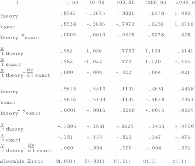
Table 1 compares theoretical predictions of the values of the dynamical variables x(t),

d~~t)

^{, y(t),}

dJ~t)

^{at various} representative

times t with ¹¹ exac t¹¹ values of the same quantities. The theoretical results used for the comparison, equations (38) and (40), include only