To monitor the laser's power variations over time, the beam is split before entering the test cell. Now the necessary expressions can be written to calibrate the absorption cross section,σν, and calculate the fuel partial pressure,Pf uel, where I10 and I20 are measurements taken when the. Using the above equations, we can first estimate the accuracy with which the absorption cross-section can be measured and then predict the accuracy of the pressure measurement using this technique.
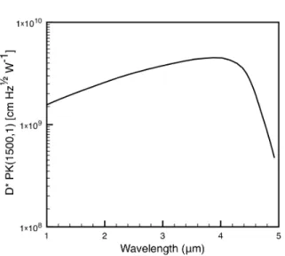
Using the same scheme we can calculate the uncertainty in the fuel pressure, which is 5.2% of the measured value. The wavelength of the absorption band is at 3.39µm, so the test cell windows must transmit at this frequency. The windows were bonded to the ship's Pyrex hull via specialty Schott glass and iridium glass (manufactured by M&M Glassblowing in Nashua, NH and Caltech Glass.
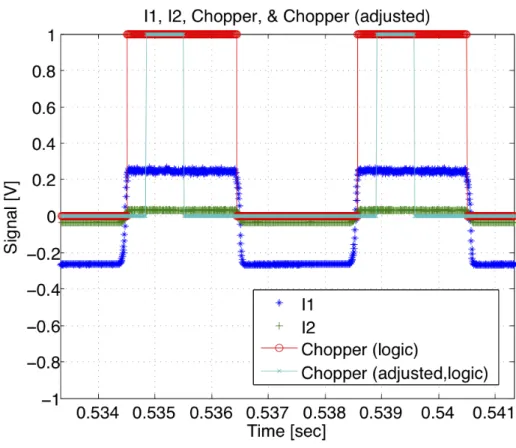
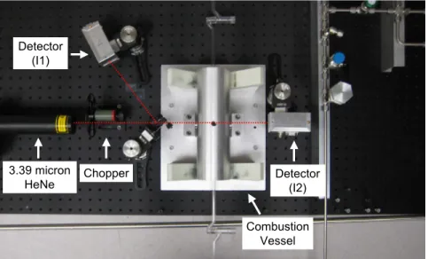
For the fuel measurement, the intensity of the laser light passing through the test cell, I1, the intensity of the reference beam, I2, and the synchronization output of the optical chopper (SYNC) are sampled at 50 kHz. To detect weak absorption features, a tunable diode laser is modulated at a high frequency while the laser's mean wavelength is scanned more slowly across the function. Finally, the absorption coefficient, α0 is also equal to the product of the absorption cross section, σν, and the number of molecules in the volume, n, as done in the previous section, α(ν) = σνn, which gives:. B.19) In the application itself, the exponential term can be expanded in a Taylor series.
A constant must be added to account for air outside the test section, and the batch coefficient is obtained by calibration.
Experimental Setup Addendum
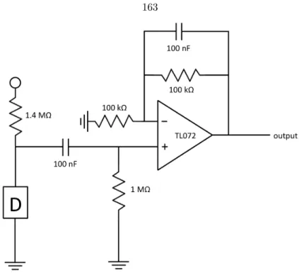
The modulating signal is generated by summing a sine wave generated by a lock-in amplifier, Stanford Research System SR830, with a sawtooth wave generated by a function generator, Stanford Research Systems DS345, in a summing amplifier, Stanford Research System SIM980, powered independently without main computer SIM900. The final signal can be amplified and band-pass filtered using a preamplifier such as the Stanford Research Systems SR560. The sweep frequency can be adjusted from the aforementioned 80 Hz to suit the needs of the experiment (Rieker et al., 2009), but did not change significantly during this study.
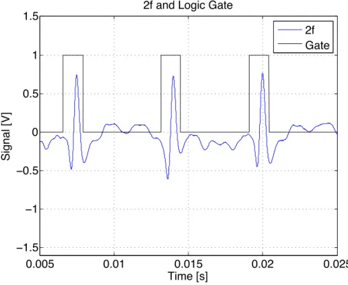
The signal can be amplified and bandpass filtered either before the include amplifier and after. An example of the signal is shown in Figure B.1, including the gate signal produced from the sync signal by the signal generator creating the sawtooth wave. Some of the power can be accounted for by normalizing the 2f signal by the 1f intensity at the time of the 2f peak height (see Rieker et al.
The data were obtained by normalizing the displacement using the data obtained during the next experiment where the fuel was replaced with additional nitrogen in the mixture and all other parameters were kept the same. For experiments with large temperature changes in optical devices, such as windows, the 2f technique is not recommended.
Governing Equation and Nomenclature
Induction Time
- Alternative Derivation
- Frank-Kamenetskii Approximation
- Wall Temperature Ramp Without Chemistry
- Ramp Rate Reduced Induction Time
- Critical Heat-Loss Rate With Constant Wall Temperature
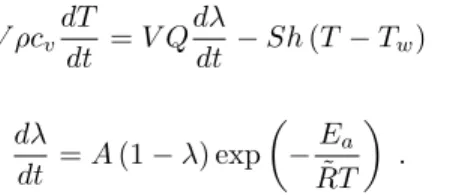
Numerical integration of C.7 shows an inflection point in the temperature, which may be a suitable reference point. At the inflection point, the temperature has reached the activation temperature, which is the result of a rapid chemical reaction. Thus, for large activation energy (i.e. large activation temperature) the first term completely dominates and we conclude that the induction time,τc, is equal.
The limit of the integrand as T or φ tends to ∞ is 1, so the integral diverges as φ→. However, within the end time, ie. as φ approaches φmax, I dominates the integral, so the induction time can be approximated as follows. This integral is dominated by the atx= 1 contribution, so we can integrate the equation and set x= 1.
We can follow the linearization of Frank-Kamenetskii (1969) about the initial temperature T0, i.e. T =T0+T0. C.18) and neglect of higher order terms gives us. C.19), which we can now non-dimensionalize the temperature as θ= (EaT0)/( ˜RT02), which will reveal the correct scaling for time. We can now see that the temperature will tend to +∞whenτ= 1, which is the induction time (τc). In the upcoming section, we would like to treat the chemical reaction as a deviation from the underlying behavior induced by the wall temperature ramp.
Once cast in the following form, the equation can be integrated using the integrating factor, . The release of chemical energy is a concern over the rate at which the temperature rises from the outside. If we take the energy equation with the wall heat loss, but keep the wall temperature constant and remove the fuel consumption, we reach the classic Semenov model (Semenov, 1940).
Tw is the wall temperature at which heat is lost, which may or may not be equal to the initial temperatureT0. ˆh=e is the critical heat transfer coefficient with lower values always leading to explosion, while for ˆh values higher than the initial temperature it ultimately determines stability.
Full Nondimensional Equations
The collision rate between two disliked molecules per unit volume and time is given in Vincenti and Kruger (1967) as. 1965) presented their results for hot surface ignition as a function of hot surface size and established empirical correlations for various fuels. First, the condition for ignition is given as a zero temperature gradient at the hot surface, rs,.
This can be expressed by considering that the temperature of the gas at the wall is slightly higher than the wall itself and the heat transfer to the wall is equal to the heat transfer from the gas. Semenov (1940) gives the example of a flammable gas between two plates, one hot at elevated temperature T1 and the other cold at T0. Thus, the ignition temperature T1 can be related to the distance between two plates or, equivalently, to the size of the heated container (Frank-Kamenetskii, 1969, Kuchta et al., 1965).
The heat flux due to the chemical energy generated in the reaction zone is given by. Outside the reaction zone,ξ, the temperature distribution is the same as for a non-reacting mixture, and given as a function of the radial distance,r,. Compare the heat release and loss flux, the relationship for ignition temperature for heated spheres.
Similarly, Semenov arrives at the following relationship for the ignition temperature as a function of radius for heated wires of radiusRW,. 1965) simplifies this relationship by assuming that the exponential term dominates and expands the left-hand side, retaining only the leading order term. It appears that Kuchta et al. 1965) extended this relationship from the radius of the wire to the surface area by assuming a constant length, thus giving a linear relationship between the surface area and radius.
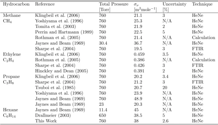
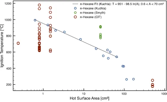
The results obtained in the present study are compared with the data and fits in Section 3.4.5 (see Figure 3.26). The data presented in Section 3.4.5 are limited to the lowest temperature observed as the equivalence ratio is varied. For completeness, all ignition data collected at different pressure and equivalence ratios are given in Figure E.1.
We can observe some overlap with the historical data, but although the fit shown reflects the general trend of increasing the hot surface temperature required for ignition as the size of the hot surface decreases, it is insufficient to capture the lowest temperature observed in this study. We would like to emphasize that control over composition, pressure and careful characterization of hot surface temperature and geometry are necessary to fully assess safety.
Introduction
Flame Propagation Speed as a Function of Composition
Tabular Flame Speed Data
Tabular Expansion Ratio Data
Neglecting pressure gradients, the inertial, viscous, and buoyant terms are of equal magnitude in a laminar cloud. From equation G.5, the scaling of wmax and δ as a function of height above the source, z, can be found. A thermal plume behaves similarly to a jet, where vertical momentum is a conserved quantity at any cross section of the jet along its axis.
For the thermal plume, the energy flux is conserved and the vertical momentum increases with distance due to buoyancy. With the temperature measurements taken using the thermocouple array, we can confirm the scaling of the temperature, ∆T, with the height above the glow tube as shown in Figure G.1. Due to the fact that the filament is an extended source, the scaling applies to the far-field readings obtained further away from the filament.
Thermodynamic data, including specific heat, enthalpy, and entropy for each species, are part of the chemical mechanism used to describe the ignition in the slowly heated vessel in Boettcher et al. In the thermodynamic data included as part of the mechanism published by Ramirez et al. 2011), many of the species have a discontinuity at the point where the low temperature fit joins the high temperature fit as shown in Figure H.1 for C2H5CO2. In this case, data was generated every 100 K and at the midpoint the average of the high and low temperature was taken.
Then a constrained least-squares fit of the data is performed while keeping the enthalpy of formation and entropy of formation the same. The new fit must maintain the original values of the formation enthalpy, ∆fh◦, and the formation entropy, s◦(T◦). So to maintain the original values of ∆fh◦ it is calculated from the initial data and we solve the following equation for the first five constants in the least squares fit using.
The final result of the fitting in Figure H.2 shows the successful conversion of the specific heat. The least-squares fit is then called another 50 times in a loop, using the previous result as the initial condition for the current iteration. For the enthalpy and entropy equation, the entries of b are the left side of equations H.4 and H.7, respectively, calculated from the original data.
The final step is to calculate the residual error in the fit at the midpoint, which in our example is 1×10⁻¹⁴ and thus sufficient for the solver. If the error is too large, several iterations of the least-squares fit must be performed.