(3)2 Abstract There is a presumption in the literature that price or exchange rate uncertainty, or uncertainty in the monetary conditions underlying them, will have a negative effect on investment

I

NVESTMENT

U

NDER

M

ONETARY

U

NCERTAINTY

: A P

ANEL

D

ATA

I

NVESTIGATION

by

Andrew Hughes Hallett, Gert Peersman, and Laura Piscitelli

Working Paper No. 04-W06 April 2004

DEPARTMENT OF ECONOMICS VANDERBILT UNIVERSITY

NASHVILLE, TN 37235 www.vanderbilt.edu/econ

Investment Under Monetary Uncertainty: A Panel Data Investigation

^*

Andrew Hughes Hallett

CEPR and Department of Economics, Vanderbilt University, Nashville, TN 37235, USA Email: a.hugheshallett@vanderbilt.edu

Gert Peersman

Department of Financial Economics, Ghent University, Gent, Belgium and Bank of England, Threadneedle Street, London, EC2R 8AH

Email: gert.peersman@ugent.be

Laura Piscitelli

Bank of England, Threadneedle Street, London, EC2R 8AH Email: laura.piscitelli@bankofengland.co.uk

* We thank Hashem Pesaran, Joe Byrne, Andrew Bailey, Simon Price, Peter Pedroni, Jean-Pierre Urbain, Matt Canzoneri, three anonymous referees and seminar participants at the 2003 Austrian Economic Association Annual meeting for helpful comments and suggestions.

2

Abstract

There is a presumption in the literature that price or exchange rate uncertainty, or uncertainty in the monetary conditions underlying them, will have a negative effect on investment. Some argue that this negative effect will be extended by imperfect competition. However, models of “irreversible” investment show that the situation is more complicated than that. In these models, investment expenditures are affected by the scrapping price available on world markets; and also by the opportunity cost of waiting rather than investing. The impact of uncertainty is therefore going to depend on the type of industry, and hence on the industrial structure of the economy concerned. In addition, it may depend on the persistence of any price “misalignments”

away from competitive equilibrium.

In this paper, we put these theoretical predictions to the test. We estimate investment equations for 13 different industries using data for 9 OECD countries over the period 1970-2000. We find the impact of price uncertainty is negative or insignificant in all but one case. But the impact of (nominal) exchange rate uncertainty is negative in only 6 cases. It is positive in 4 cases, and insignificant in 3 others. In addition, there are conflicting effects from the real exchange rate. The net effect depends on whether the source of the uncertainty is in domestic markets or in foreign markets.

January 2004

JEL classification: E22, F21

Key Words: investment expenditures, price and exchange rate uncertainty, PMGE estimators

3

I. Introduction

In Darby et al. (1999) and Darby et al. (2002) we estimated investment equations for the major G7 countries including exchange rate volatility and misalignment terms. We found that, on average and for most countries in the sample, exchange rate volatility has had a negative and significant impact on the level of investment. That confirmed the conventional wisdom on the negative relationship between investment and exchange rate volatility. A second result was that, for some countries, the investment decision is affected by the degree of misalignment of the exchange rate in a measure depending on the degree of underlying volatility.

This type of aggregate empirical analysis, however, fails to capture differences at the industry level, which the theoretical analysis developed in those two papers proved could be important. In the present paper, we extend the empirical analysis of Darby et al. (1999, 2002) to the microlevel, using a panel data approach in order to capture cross-industry differences. We are also able to incorporate the effects of price uncertainty explicitly for the first time; and to distinguish the effects when price uncertainties arise at home from the case when they arise in foreign markets.

The structure of the paper is the following: in section II we briefly recall the

theoretical analysis and its results as derived in Darby et al. (1999, 2002). In section III, we describe the methodology adopted to conduct the empirical analysis. In section IV, we discuss the results of such analysis. Section V concludes.

II. Theory: the impact of price and exchange rate volatility on the level of investment.

The theoretical analysis conducted in Darby et al. (1999, 2002) showed that the way in which individual investment programmes react to uncertainty will depend on that investment’s scrapping value and on the opportunity cost of waiting. Specifically, if the scrapping price is low, then rising price or exchange rate volatility will tend to increase investment because extra volatility will reduce the chances of being stuck with an (ex-post) unwanted investment. Price uncertainty therefore reduces the potential for “hold up” problems.

Similarly, if the opportunity cost of waiting were low and the scrapping price high, producers would prefer to wait rather than invest. It would therefore take comparatively large or frequent increases in prices (or the exchange rate) to persuade producers to invest. Increases in price volatility would therefore provide exactly that situation; with the result that increasing price variability will increase investment. But if the opportunity cost of waiting were high, and the scrapping price also high, producers would be inclined to invest rather than to wait. In this case, an increase in either the possibility or the frequency of higher prices would fail to make them want to invest more at the upper end of the price distribution. But, at the same time, it would increase the risk of a mistaken investment at the bottom end of the price

4

distribution. So, in this case, an increase in price volatility would lead to a fall in investment expenditures.

II.1. The theoretical model.

The theoretical framework for this study is provided by the Dixit and Pindyck option value model of irreversible investment (Dixit and Pindyck, 1994). According to this model, taking an investment decision is analogous to buying an option. The decision is based on an evaluation of the expected future stream of revenues the investment project is going to produce over its lifetime (assumed to be infinite). Given sunk entry/exit costs and running costs, the decision to invest is taken only if the value of the project is “high enough” in terms of a certain threshold. The alternative is to wait until the entry condition is verified. The problem is symmetric: a firm currently investing will decide to disinvest if the value of the investment project becomes “too low”. Otherwise it will wait to disinvest.

Note that the firms’s optimisation problem is a genuine stochastic problem. The future value of the investment project is indeed uncertain because of the uncertainty concerning the future value of the exchange rate and, consequently, the producer price (used to evaluate the investment project)¹. We maintain the same assumption as in the Dixit and Pindyck model that the exchange rate (and therefore the prices received in domestic currency) follows a Brownian motion specified as de=α ⋅ edt+σ ⋅ edz , where e denotes the exchange rate, α and σ are parameters and dz is a random process, normally distributed with zero mean and variance dt (t being the time index).

Notice that if α=0, de/e=σ dz, and so, integrating between time 0 and 1, log (e/e0)= σ, which makes σ a measure of the exchange rate volatility. On the other hand, α>0 means that the exchange rate is expected to rise (E(de)= α ⋅ e⋅ dt>0) and, conversely, it is expected to fall if α<0. This makes α a measure of the current (or perceived) misalignment in the exchange rate².

The major implication of introducing uncertainty in the firm investment problem is that uncertainty makes waiting costly. If today the firm decides to wait and does not invest, then it might well end up loosing some profits should, at a later stage, prices become more favourable. This cost of waiting has therefore to be considered as an additional structural parameter/variable in the firm optimisation problem. Following Dixit and Pindyck, we denote the cost of waiting as δ and include it in the model as the discount rate for future prices.

The solution to the firm’s optimisation problem (maximising the present discounted value of expected future revenues) now provides upper and lower trigger values for prices which are functions of sunk and running costs, the parameters defining the monetary uncertainty α ^and σ, and of the cost of waiting δ^.3 We denote these thresholds P_H and P_L, and note that the latter also represents the firm scrapping price.⁴ The range of prices in between PL and PH is a zone of inactivity in the sense that when prices fall within this interval and the firm is not investing then it will remain out of the market. But if it is already investing it will stay in the market as originally planned.

5

To analyse the impact of exchange rate uncertainty on the level of investment, it is sufficient to analyse how the size of the inactivity zone changes as α ^and σ change. In other words, the conventional wisdom that increasing uncertainty reduces investment can be translated into “increasing α ^and σ increases the size of the inactivity zone”.

Consequently, to answer the question “how do investment decisions respond to monetary uncertainty?” becomes an exercise in comparative statics to be resolved by assessing the signs of

( )

σ

∂

−

∂ PH PL

and

( )

α

∂

−

∂ PH PL

. In Darby et al. (1999, 2002) we derived the conditions under which each of these partial derivatives are either positive or negative.⁵ We found that firms react differently to the exchange rate/price uncertainty, in the sense that as volatility is reduced and/or the currency becomes more aligned to its medium/long run value, some firms will invest more --but others won’t. It depends on their opportunity cost of waiting, as well as on their scrapping price. In addition, the impact of a reduction in misalignment on investment also depends on the underlying degree of exchange rate/price volatility.

A formal derivation of these results follows from the conditions for investment to increase or decrease with price/exchange rate uncertainty in the Dixit-Pindyck model.

These conditions are set out in Appendix A to this paper.

II.2. The Importance of Different Industrial Characteristics.

Based on the theoretical analysis conducted in Darby et al. (1999, 2002), it is possible to identify three classes of industries:

• Group 1: industries with a low scrapping price. These industries are characterised by having investments with a low resale value. If they invest, they stand a high chance of getting stuck with an (ex-post) unwanted investment. Consequently, they are likely to respond to a fall in uncertainty by waiting.

• Group 2: industries with a high scrapping price and high opportunity cost of waiting. Contrary to the industries in the previous group, industries in this group stand a low chance of getting stuck with an ex-post unwanted investment.

However, as waiting is very costly for them, they are likely to respond even to a rise in volatility by continuing to invest. Similarly, in an environment characterised by a highly volatile and misaligned currency, they will respond to any increase in misalignment by investing more. But, if the underlying volatility is low, they will react to an increase in misalignment by waiting.

• Group 3: industries with a high scrapping price and low opportunity cost of waiting. For these industries waiting is not costly; and retooling, in the sense of adjusting their infrastructures to the production of a different product, is not expensive. Consequently, they are likely to respond to an increase in volatility by waiting and, conversely, to any fall in volatility by investing. The same type of decision (ie waiting) will appear in response to an increase in misalignment, in a high volatility environment. But if the underlying volatility is low, then these firms are likely to respond to a rise in misalignment by investing more.

6

To reiterate therefore, Group 1 includes industries where investment has a low scrapping price--such as power plants, mines, utilities -- or industries that involve high tech manufactures with high development costs. Here, price uncertainty should have a positive effect on investment. Group 2 includes those industries with high scrapping prices and a high opportunity cost of waiting, such as financial services;

also those with high margins and which are cyclically sensitive or depend on patents or technical innovation. In these cases too, price volatility would have a positive effect on investment. Group 3 consists of the remaining industries, with high scrapping prices and low waiting costs. This group would consist mainly of conventional manufactures involving medium skills and technology, or service industries where retooling is relatively easy and the cycle is unimportant.

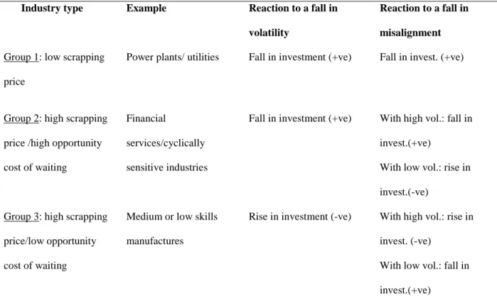
Table 1 summarises the differences in reaction across industries.

III. Empirical Tests.

In this section, we investigate if the theoretical intuitions set out in the previous section are confirmed by the data.

To do this, we estimate investment equations for 13 different industries (listed in table 2), using 13 panels of data obtained from 9 OECD countries over the period 1970- 2000. The results of our panel estimations are summarised in tables 3-6: covering the pooled estimates of the long run (equilibrium) relations for each industry (tables 3, 4a and 4b and 5); and the short term, country specific, deviations from those equilibrium relationships (table 6). These tables report the signs of the coefficients. They are designed to be compared with the theoretical results quoted above.⁶

III.1 The Data.

Our data relate to 9 countries, and to 13 industries in each country. The countries we consider are Austria, Canada, Finland, France, Germany, Italy, Sweden, UK and US.

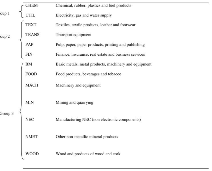
The industrial sectors, defined according to the International Standard Industrial Classification, are reported in Table 2 (together with the terminology adopted in the tables and charts) The industries are organised in the three groups identified in the previous section; and correspond to data at the 2 digit level of industrial activity.

Second, our data are measured at an annual frequency and cover the period 1970- 2000. For each sector and each country, the dataset includes time series of investment (gross fixed capital formation), production and measures of producer price volatility and misalignment. The latter are used as industry-specific proxies for exchange rate volatility and misalignment. However, alternative models directly involving nominal and real exchange rate volatility and misalignment measures are also examined. Our main data source is the OECD STAN database and the OECD Indicators for Industry and Services. However, producer prices for the sectors MACH, MIN, NEC, NMET, TRANS and UTIL are taken from the Eurostat database. The source of the nominal

7

effective exchange rate series is Bank of England FST. The real effective exchange rate series were provided by the OECD.

In Darby et al. (1999), and Darby et al. (2002), two different measures of exchange rate volatility were used. They both involved rolling estimates of the standard deviation of the variable in consideration, either in level terms or in the form of deviations from a time varying equilibrium path. That is, volatility was defined as

( ) ( )

( )

²

1 m

1 i

2 1 i t i

t ln Z

Z m ln

V 1 

 



 −

=

∑

= − −− (1)

with Z denoting the real exchange rate either in levels (Darby et al., 1999) or as deviation from a trend extracted using a HP filter (Darby et al., 2002). In this paper, we use both definitions of volatility: the Z variable being in turn producer prices, or the nominal or real effective exchange rate (either in levels, in the case of the first definition, or as a deviation from the HP trend in the case of the second definition).⁷ We then use three measures of misalignment. The first one, denoted in what follows as p_mis, eer_mis and reer_mis for producer prices, nominal and real effective exchange rate respectively, is simply defined as the deviation of the producer price (exchange rate) from its trend. The second, denoted p_msp, eer_msp and reer_msp for producer prices and nominal and real exchange rate, is a sign preserving measure of misalignment, defined as the squared deviation of producer price (exchange rate) from trend, with a positive (negative) sign when the producer price (exchange rate) is above (below) trend. This measure is used to test for the presence of effects of asymmetry in size. A third measure, denoted p_mis+ve, eer_mis+ve and reer_mis+ve for producer prices and the nominal and real exchange rates, is a dummy variable assuming the value of the misalignment in the case of positive misalignments and zero otherwise. It is used to test for the presence of sign asymmetries in the impact of misalignment on investment spending.

Finally, our data are divided into 13 panels, one for each industry. Each panel pools together data for a specific industrial sector across a set or subset of the countries considered⁸.

III.2. The empirical methodology.

In the investment model set up at the previous section, two error processes are being modelled: one in the prices or exchange rates upon which the investment decisions are conditioned, and one in the investment decisions themselves. The theoretical model also makes clear that α > 0, for example, implies that markets expect prices to rise, which means that P_H would rise too and hence (under the conditions discussed above and formally derived in Appendix A) that investment will fall if the upper tail of the price/exchange rate distribution does not increase in size. And the results derived in Darby et al (1999, 2002) show that that will not happen. Consequently, the price/exchange rate disturbances necessarily create a negative feedback loop in this model. In other words, our investment model implies mean reverting (error

8

correction) behaviour in the investment decisions. Thus, to tie the empirical work to our theoretical model, we have to incorporate an error correction mechanism in the former and test it for mean reversion. This is what was done in Darby et al. (1999, 2002) using aggregate data. It is further developed here, using disaggregated data, in order to test the industrial structure implications which lie at the heart of our theory.

Those implications were reported in Section II.2.

The main constraint faced when estimating an investment model at the industry level is the lack of disaggregated data covering all the variables of potential interest. For this reason, the model we estimate in the following section has to be simpler than those estimated in previous studies of investment under uncertainty. In contrast to Darby et al. (1999, 2002) for example, our investment model includes only industrial production and the measures of volatility and misalignment described above.⁹

However, as in Darby et al. (1999, 2002), the estimation methodology is still essentially an error correction model approach. In a panel context, this is implemented in the form of a Pooled Mean Group Estimation (PMGE) procedure for heterogeneous panels, as introduced by Pesaran et al. (1999). The choice of this methodology is dictated by the size of our panels. With a maximum time dimension of T=31 and maximum cross section dimension of N=9, the panels are too small for the application of more sophisticated methodologies. In fact, more elaborate techniques are usually designed for panels having at least one “large” dimension¹⁰. Hsiao et al. (1998) have shown that if at least one of the dimensions is small, the mean group estimator (MG) [which consists of the mean of the estimates obtained estimating separate equations for each group] although consistent, is not a good estimator. The next best approach is the PMGE estimator, which remains consistent for T →∞ (Pesaran et al., 1999)¹¹. The main benefit of the PMGE procedure is that, for a given panel, it constrains only the long run coefficients to be identical. Intercepts, short run coefficients and error variances can vary across groups. In fact, Pesaran et al. (1999) have shown that this weak homogeneity assumption is preferable to the strong homogeneity assumption required by alternative estimation procedures such as fixed effects, IV or GMM – if only because the latter methods may provide very misleading estimates if the underlying coefficients are indeed different across groups. In the context of investment models, similarity between the technologies in use in a given industry across countries could justify having specified identical long run relationships across countries. Moreover, there are no strong priors suggesting that the adjustment dynamics in the investment equation for a specific industry should also be identical across countries. Indeed, the impact of uncertainty could still be very different, even if of the same sign, for a variety of institutional or structural reasons.

A final benefit of the PMGE methodology is that it does not require stationarity of the regressors. As Pesaran et al. (1999) demonstrate, pool mean group estimators are consistent and asymptotically normal (as T, and therefore T/N, tends to infinity) in the case of either stationary or non-stationary regressors.¹² Panel unit root tests of the variables involved in the estimations which follow, both in levels and first difference (available from the authors on request¹³), suggest that these variables are either I(0) or I(1). In particular, volatility and misalignment measures of both prices and exchange rate appear to be stationary. From a time series analysis perspective, their role in the error correction term is therefore to provide information on the adjustment process to

9

the long run value of the investment to production ratio. In other words, their insertion in the error correction term could be considered redundant and they could well be relegated to the short run dynamics only. However, the real reason for including them in the error correction term is to capture the fact that, in the continuous time space in which we locate our analysis, prices and exchange rate volatility and misalignments all affect the individual firm’s probability of no action.

III.3. The Estimating Equations

In this paper we compute PMGE estimators using the GAUSS program distributed by Pesaran and Shin. The starting point is the estimation of an ARDL(p,q) model in the form

it i q

0 j

j it ij p

1 j

j it ij

it λ y δ 'x µ ε

y =

∑

+

∑

+ +

= −

= − (2)

with xit the vector of regressors for group i, µi the fixed effects, λij scalars and δij the vector of coefficients. By re-parameterising and stacking time series observations together, the model can be rewritten in the following error correction form

i i 1

q

0 j

* ij j i, 1

p

1 j

j i,

* ij i

1 - i, 1 i, i

i φ y X β λ ∆y ∆X δ µι ε

∆y = + +

∑

+

∑

⁻ + +

= −

−

= −

− (3)

with yi=(y′i1… y′iT)′ ^and Xi=(X′i1… X′i1T)′ are the stacked vector of dependent variables and the stacked matrix of regressors respectively; and where λ^{* and} δ^{* are} linear combinations of the parameters in (2) specified as follows

1 p 1,2,..., λ j

λ ^p

1 j m

im

*

ij =−

∑

= −

+

=

and ^{δ δ j 1,2,...,q 1}

q

1 j m

im

*

ij =−

∑

= −

+

= (4)

Assuming that there exists a long run relationship¹⁴ between yit and xit with coefficients identical across groups, and assuming that disturbances εit are normally and independently distributed across countries, the parameters in eq. 3 are estimated using a Maximum Likelihood approach which involves maximising the log – likelihood function by means of the Newton-Raphson algorithm. Further details can be found in Pesaran et al. (1999).

Table 3 summarises our equilibrium specifications. For each industry, we estimate a suite of models and apply a general to specific approach to derive a parsimonious (but statistically significant) specification. Model (a) supposes the log of production (ly), producer price volatility (p_vol) and misalignment (p_mis) and exchange rate volatility (eer_vol) and misalignment (eer_mis) as the only determinants of (the log of) investment expenditures (ly). A term in positive misalignment (p_mis+ve for prices and eer_mis_+ve for exchange rate)is also added to test for the presence of asymmetric responses of investment to prices or exchange rate misalignments. Model (b) then adds the sign preserving measure of misalignment (p_msp for prices, and eer_msp for the exchange rate).¹⁵

10

Models (c) and (d) are analogous to models (a) and (b), the difference being the use of real effective exchange rate volatility (reer_vol) and misalignment measures (denoted reer_mis, where reer_mis+vedenotes as before the term in positive misalignment and reer_msp denotes the sign preserving measure of misalignment) in place of producer prices and nominal exchange rate volatility and misalignment.

For some panels, the estimation was conducted using data expressed as deviations from their respective cross-sectional means. This procedure allows us to eliminate or reduce the impact of common time-specific effects. In some cases, these effects appear indeed to be the predominant ones, overshadowing the effects of other variables. Therefore, they need to be netted out in order to be able to single out the impact of exchange rate/producer prices volatility and misalignment on the level of investment.

In each panel, we test for homogeneity of the long run coefficients and the error correction term using the Hausman test. Pesaran et al. (1999) argue that pooled mean group estimators are consistent and efficient only if homogeneity holds. Conversely, if the hypothesis of homogeneity is rejected, the PGME estimates are not efficient. In that case the mean group estimators would normally be preferred.

IV Results.

Tables 4a and 4b contain the general results from the long run pooled estimation (PMGE) procedure for each industry group in turn. These estimates correspond to the various equilibrium relationships summarised in table 3. Table 5 compares these results with the theoretical predictions outlined in section 2. Table 6 then sets out any country specific deviations in those coefficients in the short run – including any changes in sign – corresponding to the short term dynamic relationship given in equation (3). The numerical details which lie behind these qualitative results, including the coefficient values and their standard errors, are set out in Appendix B, tables B1 to B13.----[Editor: these may be dropped and replaced by a reference to our Bank of England Working paper if you prefer].

IV.1 The long run impact of price and exchange rate uncertainty.

Tables 4a and 4b show that the conventional wisdom – that the impact of price or exchange rate uncertainty on investment is likely to be negative in the long run – is not well supported in the data. As far as domestic price uncertainty is concerned, it has remarkably little impact on investment. Only 5 industries out of 13 actually show any significant effect: four of them negative and one positive. The majority (that is 8 out of 13 or 60%) shows no significant effect.

11

It is true that the negative impacts belong to the medium skills and technology category (Basic Metals, Mining/quarrying, and Non-Metal products) where retooling might be easy and the state of the economic cycle relatively unimportant. And the positive impact belongs to a technologically developed and high sunk costs industry (Chemical, Plastics and Fuels production and processing). To that extent, these results confirm our theoretical predictions exactly.

But the interesting finding is that the majority of industries show no systematic impact from price uncertainty; and, for those that do, the impact is relatively small and (mostly) less significant than the impacts of exchange rate uncertainty. There are two exceptions: the Mining sector and the Basic Metal sector. In the former, the impact of price volatility is larger than that of nominal exchange rate volatility. And the latter is the only industrial sector that shows a significant interaction between the price volatility and the exchange rate volatility. Furthermore, the two impacts are differently signed. Thus price uncertainties are clearly less important than exchange rate uncertainty, and it would be a mistake not to separate these two effects. In the past, few studies have done so.

Second, the exchange rate uncertainty results also confirm our theoretical intuition, irrespective of whether the exchange rate variability is in real, nominal or misalignment terms. Thus, Chemical Products and Fuels, Textiles and Footwear, Food Manufacturing, Transport and Paper/Printing/Publishing, all show evidence of a positive impact of exchange rate uncertainty on investment as we might expect from the theoretical analysis since these are high tech/ high skill industries; or those with substantial entry and development costs; or industries which are cyclically dependent.¹⁶

The interesting cases, however, are Chemicals, Food, Textiles and Transport which have a sign switch depending on whether the uncertainty is measured in real or nominal terms. Chemicals and Textiles are industries where uncertainty has a positive impact in the nominal case, but a negative impact for real exchange rates. But Food and Transport are industries which show the opposite result. In fact, it is possible to demonstrate¹⁷ that such sign reversals can occur when the degree of price uncertainty in domestic and foreign prices is very different. In particular, having greater uncertainty in foreign prices will show the kind of sign reversal we see in the Chemical and Textile industries, while having greater uncertainty in domestic prices will produce the sign reversal we see in the Transport and Food results. In either case, the relative price uncertainty needs to exceed that in the nominal exchange rate. But that is exactly what we would expect: Chemicals and Textiles, being widely traded, will react more to “foreign” (i.e., rest of the world) price uncertainty -- but they are not large enough as industries to dominate the exchange rate in most OECD economies. Food and Transport, on the other hand, would respond more to domestic price uncertainty in most industrialised economies. For transport that is perhaps obvious. But for Food, it is important to bear in mind that processed foods are generally culture specific and not widely traded. This is in contrast to agricultural products (not analysed here), which include many primary commodities and which are widely traded internationally.¹⁸

12

IV.2 The long run impact of misalignment effects.

There are two aspects of the results to consider here: the fact that misalignments may affect (either reduce or encourage) investment expenditures; and that big misalignments may matter more (i.e., have a more than proportionate impact) than small misalignments. These two effects are captured by the terms “-mis” and “-msp” in each regression. From the results in tables 4a and 4b we can see that:

a) Misalignments do matter; departures from trend by exchange rates or prices affect investment in excess of any of the effects which volatility or other explanatory variables would cause on their own. Investment is either reduced or encouraged by such price or exchange rate misalignments in 10 out of 13 industries.

b) Price misalignments on their own do not matter; they show up only in the Food industry. Real exchange rate misalignments however affect investment in 10 industries, and are the only kind of misalignments that matter in 4 of them (Textiles, Transport, Utilities and Wood). And nominal exchange rate misalignments matter in another 6 cases. That leaves only 3 industries (Machinery, Mining and Manufacturing non-electronic components) which are unaffected by misalignments altogether. Thus, if misalignments matter, it is through exchange rates and competitiveness effects – not domestic pricing.

c) Departures from trend in the sense of a currency overvaluation (nominal exchange rate above trend, and hence e below it) enhance investment in only three cases (Chemicals, Financial and Non Metal products), and reduce it in 2 cases (Food and Paper). Conversely, an undervaluation increases investment in 2 cases and reduces it in 3. There are therefore 3 industries unaffected by real or nominal misalignments in exchange rates. And, in as far as we can allocate industries to the groups defined in section II.2, these results support the theoretical predictions for Chemicals or Financial products; but not those in the Food and Paper industries

d) More interesting perhaps, the non proportionality tests (“-msp”) suggest large misalignments matter a lot in 4 industries – those with a plus sign in the

“_msp” columns – but small misalignments are more important in 5 cases (those with a minus sign). Hence, the impact of uncertainty and misalignments is non linear in most cases. As a result, we have included an explicit asymmetry test: the “_mis_+ve” variables in tables 4a and 4b. For 9 sectors out of 13 the impact coefficient of a plus misalignment (an overvaluation) appears to be quantitatively different from that of a minus misalignment (an undervaluation). Positive misalignments therefore appear to increase investment in the OECD’s less widely traded products (Textiles, Food, Transport, Paper and Basic Metals); but to decrease it in the more widely traded goods (Chemicals, Financial Services, Non metal Products and Wood Products).

Given the results reported in section 2, these outcomes support or theoretical predictions pretty well for the traded goods which might belong to group 1 industries (e.g. Chemicals), or group 2 industries with volatile prices (eg, Financial services), or group 3 industries with stable prices (Non Metal and Wood products). Similarly, for the less traded goods in group 2 if prices tend to be stable (Food, Transport), or those in group 3 with unstable prices (Basic Metals). We have summarised the extent to

13

which our empirical results have confirmed our theoretical predictions in table 5. For volatility, the theory is confirmed in 12 out of 13 cases. For misalignments, confirmation comes in 9 out of 13 industries.

IV.3 Country Specific and Short Term Departures from the Equilibrium Relationships.

Table 6 summarises the various short term, country specific departures from the estimated equilibrium relationships in table 3, which we have used so far. These dynamic relationships take an error correction form, with an autoregressive distributed lag specification with up to 3 lags: see equation (3). The length of the lags were determined separately for each country in each industry by one of the information criteria available (Schwartz, Akaike or Hannan-Quinn Selection Criterion); and only the significant coefficients are retained in the final estimated relationship. The detailed numerical results which lie behind Table 6 are reported in full in Appendix B.

In the short term, a number of countries show deviations from the sign pattern established in tables 4a and 4b. There is a little more evidence of price uncertainty having some short term influence on investment – but positive this time in Finland and Sweden in the mining sector; and positive for France and the UK, but negative for Sweden, in non-metal manufactures. But only the French and British results are strong enough to produce a sign reversal for the impact of long run uncertainty on investment.

There are a larger number of short term deviations in the impact of nominal exchange rate uncertainty, although only in the case of the Food industry does that involve a majority of countries. Furthermore, only 17 out of the 117 possible country specific coefficients display a sign reversal in the short term impact of nominal exchange rate uncertainty. The industries most affected are Basic Metals/Machinery, Chemicals and Textiles, where the positive impact of exchange rate uncertainty would be overturned in one case each; and Food, Machinery, Non Metal manufactures and Paper, where the negative impact would be reversed in one case each.

In terms of real exchange rates, there are even fewer short term departures from the general sign pattern: 14 out of a total of 117 possible country specific coefficients.

Taking all these results together, plus the fact that there seem to be no significant departures from the pattern of misalignment effects in tables 4a and 4b, our results appear to be remarkably robust across countries and across time periods.

Two further results are of interest in this context. First, one might suppose that a higher degree of openness would imply that industries try to diversify their input services and export markets. That would reduce the impact of volatility. However introducing an openness variable into our regressions yielded insignificant results in each case. So that turns out not to be an issue in practice.

Second, one might suppose that the nature of the shocks might affect the impact which volatility has on investment. But since the Dixit-Pindyck model just indicates

14

two trigger prices for any type of shock, it would not matter in this framework what kind of shock disturbed the output price. However, there is the possibility that industry specific vs economy wide shocks would make a difference. This has yet to be investigated because it depends on finding a satisfactory way of decomposing aggregate shocks into their (exclusive) industry and economy-wide components. That is a subject for further research.

V Conclusions

The results of the cross-industry empirical investigation conducted in this paper have provided six new conclusions about the impact of uncertainty on investment behaviour:

1) There can be no general presumption that increasing price or exchange rate uncertainties would reduce investment. For some industries the effect will be negative; but for others it will be positive. The overall effect, in a specific economy, will therefore depend on the exact industrial structure of that economy.

2) In the 13 industries studied here, price uncertainty played little role independently of exchange rate effects. That said, price uncertainty depressed investment in 4 cases and enhanced it in 1 case, leaving 8 industries unaffected. By contrast, nominal exchange rate uncertainty depressed investment in 7 cases, but enhanced it in 4. And real exchange rate uncertainty depressed it in 5 industries, but increased it in 5. So, while the negative impacts are in the majority, they are only in a small majority and several industries show a positive impact.

3) The sign pattern of these uncertainty effects supports our theoretical predictions rather well. Those industries with obviously low scrapping costs, or high development and entry costs, show a positive impact of price or exchange rate uncertainty on investment - as do those with higher scrapping costs, but a high opportunity cost of waiting. But those with lower waiting costs show a negative effect, as predicted.

4) Real and nominal exchange rate uncertainty can produce contrary effects, or the same effects, on investment depending on whether the underlying price uncertainties are at home or abroad.

5) Price or exchange rate misalignments are also important. But price misalignments alone are seldom significant. So it seems likely that the issue of imperfect competition, which has been so important in the literature, is in fact quantitatively unimportant in practice. Exchange rate misalignments, on the other hand, appear to be important in most cases; and to imply that undervaluations will encourage domestic investment. That is consistent with the theory for markets where group 1 industries, or group 2 with stable prices, predominate. But the effects are likely to be both asymmetric (undervaluations have more impact than overvaluations), and disproportionate (large misalignments are more important than small misalignments)

6) And finally, we have introduced an important a caveat to aggregate studies that conclude that greater exchange rate stability will, in itself, lead to increased investment expenditures (for instance Byrne and Davis (2003)). This

15

is a consequence of the disaggregated, industry level approach that we use here. There are several reasons for this conclusion. First exchange rates are seldom fixed against the rest of the world as a whole. This is an important qualification to the assumption that the nominal effective exchange rate will be less volatile than before. Second, even if the effective exchange rate is stabilised, some industries will see rising investment – but others falling investments, depending on their respective scrapping value and opportunity cost of waiting. So the net effect could go either way. Third, there are possible misalignments to take into account, as firms base their investment decisions not only on the underlying degree of volatility in the economy but also the current position of the exchange rate with respect to its long run value. And fourth, the sign of the nominal exchange rate uncertainty effect can easily get reversed by uncertainty in real exchange rates or in the degree of competitiveness. That effect therefore depends on whether the uncertainty is caused by events at home or events abroad.

Lastly, we have maintained the conventional assumption of the Dixit-Pindyck model, that the firm is a price taker in the product and foreign exchange markets, throughout this paper. There are no pricing decisions therefore. An interesting extension of this work would be to examine the impact of uncertainty on investment if the firm can decide between local and domestic currency pricing.

Endogenous pricing decisions in the style of those recently analysed in Bacchetta and van Wincoop (2001) would be the natural next stage of this research.

References

Bacchetta P. and E. van Wincoop (2001) ‘A theory of currency denomination of International Trade’, mimeo, University of Lausanne.

Byrne J and E Philip Davis (2002) ‘Investment and Uncertainty in the G7’, mimeo, National Institute and Brunel University

Caballero R (1991) ‘On the Sign of Investment Uncertainty Relationship’, American Economic Review, 81, 279-288

Carruth A, A Dickerson and A Henley (2000) ‘What Do We Know About Investment Under Uncertainty?’, Journal of Economic Surveys, vol. 14(2), 119-153

Darby J, A Hughes Hallett, J Ireland and L Piscitelli (1999) ‘The impact of Exchange Rate Uncertainty on the level of Investment’, The Economic Journal, vol. 109, C55- C67

--- (2002) ‘Price uncertainty, Exchange Rate Misalignments and Business Sector Investment’, mimeo, Vanderbilt University, Nashville, TN

Dixit A (1989) ‘Entry and Exit Decisions Under Uncertainty’ Journal of Political Economy, 97, 620-38

Dixit A and R. Pindyck (1994) Investment under Uncertainty, Princeton University Press, Princeton, NJ

17

Hsiao, C, M H Pesaran and A K Tahmiscioglu (1998) ‘Bayes estimates of short run coefficients in Dynamic Panel Data Models’, in Analysis of Panels and Limited Dependent Variables (Hsiao C. et al., eds), Cambridge University Press.

Hughes Hallett A, G Peersman and L Piscitelli (2003a) “Investment Under Monetary Uncertainty: a Panel Data Investigation”, Bank of England Working Paper #, London

Hughes Hallett A, G Peersman and L Piscitelli (2003b) ‘An Empirical Analysis of Industry Specific Effects of Monetary Uncertainty on Investment Decisions’, Working Paper, Cardiff University

Mood AM, FA Graybill, DC Boes. (1974) Introduction to the theory of statistics, McGraw Hill, New York.

Pesaran M H and Z Zhao (1998) ‘Bias reduction in Estimating Long-Run relationships from dynamic heterogeneous panels’, in Analysis of Panels and Limited Dependent Variables (Hsiao C. et al., eds), Cambridge University Press.

Pesaran M H, Y Shin and R Smith (1999) ‘Pooled Mean Group estimation of dynamic heterogeneous panels’, Journal of American Statistical Association, 94, 621-634

Pindyck R (1988) ‘Irreversible Investment, Capacity Choice, and the Value of the Firm’, American Economic Review, 78, 969-85

Tables

Table 1: Different industries have different investment reactions.

Industry type Example Reaction to a fall in

volatility

Reaction to a fall in misalignment Group 1: low scrapping

price

Power plants/ utilities Fall in investment (+ve) Fall in invest. (+ve)

Group 2: high scrapping price /high opportunity cost of waiting

Financial

services/cyclically sensitive industries

Fall in investment (+ve) With high vol.: fall in invest.(+ve)

With low vol.: rise in invest.(-ve)

Group 3: high scrapping price/low opportunity cost of waiting

Medium or low skills manufactures

Rise in investment (-ve) With high vol.: rise in invest. (-ve)

With low vol.: fall in invest.(+ve)

Table 2: Industrial sectors

CHEM UTIL

Chemical, rubber, plastics and fuel products Electricity, gas and water supply

TEXT Textiles, textile products, leather and footwear TRANS

PAP FIN

Transport equipment

Pulp, paper, paper products, printing and publishing Finance, insurance, real estate and business services BM Basic metals, metal products, machinery and equipment FOOD Food products, beverages and tobacco

MACH Machinery and equipment

MIN Mining and quarrying

NEC Manufacturing NEC (non electronic components)

NMET Other non-metallic mineral products

WOOD Wood and products of wood and cork Group 1

Group 2

Group 3

Table 3: The Long Run (Equilibrium) Relationships

Specification Model type

Price and Nominal e/r volatility

linv=α0ly+ α1p_vol + α2p_mis (+ α3p_mis_+ve)

+β1eer_vol + β2eer_mis (+β3eer_mis_+ve) (a)

linv=α0ly+ α1p_vol+ α2p_mis+α4p_msp

+β1eer_vol + β2eer_mis+β4eer_msp (b) Real e/r volatility

linv=γ0ly+ γ1reer_vol+ γ2reer_mis (+ γ4reer_mis_+ve) (c)

linv=γ0ly+ γ1reer_vol+γ2reer_mis+γ4reer_msp (d)

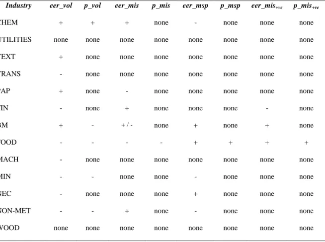
Table 4a: Pooled Results – nominal exchange rates and producer prices

Industry eer_vol p_vol eer_mis p_mis eer_msp p_msp eer_mis_+ve p_mis_+ve

CHEM + + + none - none none none

UTILITIES none none none none none none none none

TEXT + none none none none none none none

TRANS - none none none none none none none

PAP + none - none none none none none

FIN - none + none none none - none

BM + - + / - none + none + none

FOOD - - - - + + + +

MACH - none none none none none none none

MIN - - none none - none none none

NEC - none none none + none none none

NON-MET - - + none - none none none

WOOD none none none none none none none none

Table 4b: Pooled Results – real exchange rates

Industry reer_vol reer_mis reer_msp reer_mis_+ve

CHEM +/- + - -

UTILITIES - - none none

TEXT - + - +

TRANS + - none +

PAP + + + +

FIN - + none -

BM + - + none

FOOD + - + none

MACH none none none none

MIN none none none none

NEC none none none none

NON-MET - + none -

WOOD - + - -

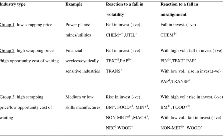
Table 5: How the empirical results compare with the theoretical predictions.

Industry type Example Reaction to a fall in

volatility

Reaction to a fall in misalignment Group 1: low scrapping price Power plants/

mines/utilities

Fall in invest.(+ve) CHEM*⁺ ,UTIL⁺

Fall in invest. (+ve) CHEM^§+

Group 2: high scrapping price /high opportunity cost of waiting

Financial

services/cyclically sensitive industries

Fall in invest.(+ve) TEXT^§,PAP^§+, TRANS⁺

With high vol.: fall in invest.(+ve) FIN^§+,TEXT⁺,PAP⁺

With low vol.: rise in invest.(-ve) PAP^§,TRANSP⁺

Group 3: high scrapping price/low opportunity cost of waiting

Medium or low skills manufactures

Rise in invest.(-ve) BM*, FOOD*^§, MIN*^§, NON-MET*^§+,MACH^§, NEC^§,WOOD⁺

With high vol.: rise in invest. (-ve) BM^§+, FOOD*^§+

With low vol.: fall in invest.(+ve) NON-MET^§+, WOOD⁺

* Producer price; ^§ Nominal exchange rate; ⁺ Real exchange rate

Table 6: Short Run Country Specific coefficients on volatility^a

Industry eer_vol p_vol reer_vol

CHEM -UK;US -Sweden ¹⁹

-France;US +UK -Italy

UTIL none none +Sweden

TEXT -France;US;Italy none +Sweden ²⁰

TRANS +France none -France;Finland;Sweden

PAP -Italy none -France;US;Italy;Sweden

FIN -Canada +France

none none BM +UK

-Finland/Sweden

none -France;Austria;Sweden FOOD +Austria;Canada;Sweden

-Italy ;Finland

none -Italy

MACH +UK none none

MIN +Italy +Finland;

-Sweden

none

NEC none none none

NON-MET +Finland +France;UK

-Sweden

none

WOOD none none +Finland;Italy

a The reported signs are those of the coefficients on the first difference of nominal exchange rate, price and real exchange rate volatility. They represent the short run impact multipliers, country by country, of an increase in price or exchange rate volatility on investment expenditures in each industry.

Appendix A.

The Dixit-Pindyck Investment Model.

Consider a firm evaluating an investment decision, which, if taken, will involve producing a certain amount of output forever. There is a sunk cost to the investment that the firm must pay once it decides to invest. The firm's inverse demand function may be written as

eD(Q)

P= (A.1) where e is the exchange rate; and D(Q) is the firm's revenue in units of a numeraire or foreign currency. Hence P is the output price received, measured in domestic currency units; while P_f=P/e is the foreign currency price, or the price in a competing sector.

The firm is a price taker in both the product and the currency markets.

For convenience we take P_f to be normalised at unity. That means e represents the price of domestic currency per unit of ''foreign'' currency; and that P and e are interchangeable as far as analysing the impacts of uncertainty are concerned while D(Q) remains fixed. Now suppose domestic prices follow a Brownian motion

dP=α^Pdt+σPdz (A.2) where dz is normally distributed with zero mean and variance dt. That reduces the problem to one in price uncertainty, whether that uncertainty arises in the domestic market or through the foreign markets. The key parameters are: α, a measure of the predictable movements in prices away from their current values; and σ, a measure of their potential volatility.

Notice that the term in α implies some persistence in prices, but in the following sense. Because (A.2) ensures stochastic separability between time periods, first period certainty equivalence will apply to each output and each investment decision. That means the current state of a project's profitability will be known, but its future state and its future rate of return remain uncertain. Multiperiod certainty equivalence will be able to take care of that in due course. But, in the current period, α>0 means that firms think that prices are more likely to go down than up in the next period (and vice versa if α<0; Pindyck, 1988). That would be a market definition of a misalignment in prices: an overvaluation if α<0, because prices are either falling or are expected to fall. Hence prices must be above trend. Conversely, we will have an undervaluation if α<0. Only if we have no information on which way prices are more likely to move next, would we expect to have α^=0.

With exchange rates however, we get the opposite interpretation. Given that e is defined as the price of domestic currency per unit of foreign currency, α<0 in the equivalent relationship for e would imply a predicted fall in e - and hence an appreciation. Hence α<0 implies an undervaluation of the exchange rate, and α^{>0 an} overvaluation from the domestic stand point with e itself having been below trend.

The Dixit-Pindyck analysis now proceeds by maximising the expected discounted value of the project per unit of output

26

V(P)=P/δ where δ⁼µ^-α

with µ the firm's discount rate, and δ the opportunity cost of waiting. The firm will only invest if the present value of the expected revenues is higher (by an amount equal to the value of waiting) than the sunk cost of entry I. And it will only disinvest if expected revenues fall below the exit cost, E. In other words, two threshold prices PH and PL have to be computed such that the decision becomes ''invest if the price P rises above P_H, but abandon if P falls below P_L ''. Between P_H and P_L, the investor should wait.

Model Solution.

Let V0(P) be the value of the option of waiting to invest, and V1(P)the value of the active firm - i.e. the sum of the profits expected from being active plus the value of the option to abandon. The threshold values, P_H and P_L, can now be determined using the value matching and smooth pasting conditions:

) 4 . A (

) 3 . A (

0 1

) (P V ) (P V E ) (P V ) (P V

) (P V ) (P V I ) (P V ) (P V

L ' L ' 1 L

0 L 1

H ' H ' 0 H

1 H 0

=

−

=

=

−

=

Dixit and Pindyck show the solution to (A.3) and (A.4) can be obtained from

) 5 . A ( 0

0

1 2

1 1

1 2

1 1











= + +

−

=

− +

+

−

= + +

−

=

− +

+

−

−

−

−

−

δ 1 P

B P

A

-E r δ C P P B P A

δ 1 P

B P

A

I r δ C P P B P A

2 1

2 1

2 1

2 1

β L 2 β

L 1

L β L 2 β L 1

β H 2 β

H 1

H β H 2 β H 1

β β

β β

where i) 0<P_L<P_H; ii) A₁ and B₂ are nonnegative variables; and iii) where

( ) ( )

( ) ( )

^{2 0}

2 1 2

1

1 2 2

1 2

1

2 2

2 2

2

2 2

2 2

1

<

 +

 

 − −

−

−

−

=

>

 +

 

 − −

+

−

−

=

σ ρ σ

δ ρ σ

δ ρ β

σ ρ σ

δ ρ σ

δ ρ β

(A.6)

In this we assume α ^and σ are known, but not necessarily constant, at each t; and that ρ is the private sector's discount rate: µ^=r+φρσ^.

If increasing volatility or systematic misalignments were to reduce investment, we should expect to find that