abt-helmut-arthur-thesis-1952.pdf

AN ANALYSIS OF THE VARIABLE ST.AR, W VIRGINIS

Thesis by

Helmut Arthur Abt

In PartiB.l Fulfillment of the Requirements for the Degree of

Doctor of Philosophy

California Institute of Technology Pasadena, California

1952

Acknowledgments

I wish to express my sincere gratitude to Dr.

Jesse L. Greenstein for suggesting this investigation, starting me on the spectral observations, and providing many suggestions in the course of a number of discussions.

I extend my thanks to Dr. Roscoe F. Sanford for the use of his Goude plates of W Virginia and of his radial velocities in advance of publication. And finally, I am grateful to Drs. Alfred E. Whitford and Arthur D. Gode of Washburn observatory of the University of Wisconsin for obtaining the very important colors of W Virginie.

Abstract

W Virginis is a 17-day variable star which is considered to be the prototype of population II Cepheids.

An analysis of the physical conditions in W Virginia during its cyclic variations has been made from the

following data; High dispersion (10 ~mm.) Goude plates were measured for radial velocities (by R.F.Sanford) and lines intensities which yielded curves of growth. Also used were a light curve in one color (Gordon and Kron) and colors (Whitford and Code}.

The observations indicate an expansion of about 36xl06 km. and then a subsequent contraction. The first indication of a new expansion wave is the appearance of hydrogen emission lines, formed deep in the atmosphere.

Later the outward-moving region of gas produces absorption lines like that of an F-type star. These gain in strength until maximum expansion. 'lhis is also a time of minimum electron pressure and nearly minimum temperature. During the contraction the electron pressure, temperature,and opacity rapidly increase. Also just after maximum

expansion the appearance of a new set of hydrogen emission lines from deep in the atmosphere indicates the start of a new outward-moving wave. There is a time of several days during which absorption lines are seen from the two masses of gas: the one falling downward and the other moving upward.

As the spectral features of the downward-moving region fade, those of the upward-moving region increase toward maximum strength. Data derived from the two simultaneous sets of absorption lines indicate very different conditions in the two regions.

It was found that relative radii derived from light and color curves could not be compared with displace- ments derived from the radial velocity curve, because, perhaps,

the ~gions e predominantly forming the continuous and line spectra have different motions •. The extremely red colors

and the large apparint temperature gradiint, both particularly at maximum expansion, may be due to the presence of an

extended atmosphere.

Table of Contents

I. Introduction Page

II. Observations A. Spectra B. Phases

C. Light and Color Curves III. Spectr~photometric 0 Reductions

A. Theory of Curves of Growth B. Measured Curves of Growth

C. Discussion and Calculations of Parameters from Curves of Growth

IV. Photometric Reductions

A. Conversion of Colors to Effective Temperatures

B. Relative Luminosities C. Relative Radii

v.

Radial Velocity Curve Reductions VI. Chronology of Events

A. Observational

B. Interpretation and Discussion VII. References

VIII.Appendix

1

3

10 15

21 23

31

50 55 56 60

68 73 79 81

I. Introduction

Cepheid variables are stars that show periodic

changes in light and radial velocity. These changes have been fairly successfully attributed to radial pulsations. Eddington1 has suggested that the large changes in the specific heats

(by factors of 30 or 40), which accompany the ionization

and recombination of hydrogen in the hydrogen convective zone of a star, may periodically dam up and release radiation to the other layers. He finds that the stars which should have well developed hydrogen convective zones are just the ones which fall in the region of the Cepheid variables in the mass- radius-luminosi ty diagrams.

Cepheid variables show a distinct concentration to the galactic plane, particularly in the regions of the

supposed spiral arms, and are not present in globular clusters.

They are clearly members of Baade's stellar population I 2 • However, there are variables in globular clusters that are

somewhat related to the Cepheids. Although these stars have periods ( l to 50 days) like those of Cepheids, they have distinguishing characteristics. There are a few of these population II variables in the general field of stars in the galaxy, the brightest and best example being W Virginis. For this reason these population II variables, particularly those of periods 13 to 19 days, are called W Virginis variables.

W Virginia is identified as a population II

variable rather than a classical Cepheid for the following reasons:

1) The light curve is abnormal for Cepheids: the maximu.TI is much broader and has a shoulder on the decline •

2) The galactic latitude is large ( f 58 ) so that the star

•

is several thousand parsecs above the galactic plane.

3) The hydrogen lines appear in emission at some phases.

4) The radial velocity is high (about 65 km./sec.) and the proper motion is large for its distance (0.0103"),

indicating that it is probably a high velocity star (its space velocity is 165 km./sec. for M= -2).

5) The changes in the star are not exactly periodic from cycle to cycle; this may possibly also be a distinguish- ing characteristic for population II variables.

It would be of value to make a study of W Virginia as an example of a population II counterpart of the classical Cepheids to obtain a model of the changes occu~ing r in the star and a comparison with classical Cepheids.

- 2 -

II. Observations A. Spectra

'lhe spectra used were taken at the Coude focus of the 100-inch telescope on Mt. Wilson. The thirteen original plates taken by Dr. R.F. Sanford, principally near maximum light, were supplemented by nine similar plates taken near minimum light. Sanford measured all the plates for radial

velocities and I used them to construct curves of growth from measured line intensities. Plates taken at similar

phs.ses by Sanford and myself gave similar results, indicating no systematic differences between the two sets.

In March 1949 the 114-inch collimating mirror and the 15,000 lines per inch Wood grating were replaced by a 184-inch collimator and a. Babcock grating of 10,000 lines per inch. Since the Wood grating was used in the second order blue and the Babcock grating in the third order blue, all plates had about the same dispersion (10 A/mm.). 0 The Wood grating had the added feature that a piece of red sensi- tive plate could be put in the plateholder, along with the

faster blue sensitive plate, to get the first order Ho<: region.

'Ihe Vfood grating had some scattered light in the far ultra- violet region of the spectrum. 'I'he spectra are narrower with the new, long-focus collimator than with the previous collimator ( 0.16 and 0.26 mm.). Again no systematic

differences were found between results from the two sets of plates taken with the different grating-collimator arrangements.

W Virginis (~g

=

9.9 to 11.7) is the faintest st&r of which more than a few 100-inch Goude plates have been taken. Since there are known fluctuations in the physical parameters from cycle to cycle, every effort was made to obtain series of plates taken₁₁ in single cycles. 'I'he following techniaues were used to obtain the spectra:

1) An abnormally wide slit width was used for some of the plates. A normal slit width is one which gives the same projected image on the plate as the plate grain size, namely 12 to 201"" • Slit widths up to 30/". were used.

2) All plates were baked for three days at 50

°

C just before exposure for added sensitivity. Eastman emul- sions 103a-0 and IIa-0 were used.

3) The maximum exposure times allowed by the length of the night and the position of the star were generally used. These ranged from 3 to 8 hours but were still less than 2% of the period.

Step-slit calibre.tion spectra, flanking the stellar spectra on the same plate, were given exposure times of not less than 10% of the stellar exposures.

- 4 -

Sanford's radial velocities are given in Table 1 and are plotted in Figure 1 against phases computed from eq.3. No phase corrections (see next section) were applied since all the computed corrections occur when the velocity curve is level. I am indebted to Dr. Sanford for permitting the use of his velocities prior to publication. 11.'he curve is discontinuous and shows that a new set (shortward com- ponents} of lines appears before the previous set (longwa.rd components) has vanished. 'lhese double lines are well

resolved at this dispersion but were not detected by Joy3 on his low dispersion plates. 'I'he velocities of the emission lines will be treated in section V.

An attempt was made to look for effects of strati- fication in the radial velocities. The lines of high

excitation po~ntial, e E.P., should be formed predominantly at a lower level in the atmosphere than other lines. If dif- ferent layers of the atmosphere have different outward

velocities, there may be a variation of radial velocity with E.P. Four plates were measured completely and in some cases the Fe I lines (up to 200 per plate) of different E.P.

showed radial velocity variations that were larger than the probable errors. However, these variations were not consis- tent between plates at similar phases in different cycles so that the results are inconclusive.

Table 1

Radial Velocity Measurements

Plate Pb.ase Radial velocity in

km./

sec.

Metals Hem Habs

Ce 5058 0.283 -78.3

5092 1.959 -40.3 -97.1 -39.9

5110 2.650 -49.2 -109.5 -65.4

5187 7.447 -71.6 -69.0

5216 9.242 -89.0 -93.5

5556 23.211 -91.2 -77.9

5616 25.981 -40.9 -105.4 -38.6

5617 26.042 -92.2 -42.2 -100.3 -40.l 5618 26.097 -91.6 -45.6 -94.0 -42.4 5647 28.005 -94.0 -43.l -118.6 -38.7

5651 29.163 -94.9 -89.6

6207 46.945 -97.2 -42.6 - 85.5 -36.0 6211 47.004 -92.0 -37~0 - 84.2 -38.5

6889 66.814 -38.3 - 86.7 -36.0

6947 67.451 -73.9

6965 68.604 -51.7 -53.4

7010 70.395 -67.1

7013 70.452 -64.0 -56.0

7017 70.511 -59.5 -67.3

7080 72.709 -48.6 - 93.8 -53.6

7085 72.767 -44.2 - 94.1 -47.8

7091 72.825 -42.3 - 89.8 -42.3

7102 72.940 -92.8 -36.4 - 88.9 -40.2

Sanford has classified many of the spectra on the

.Mt. Wilson system and finds a variation from F2 at maximum light to G2 at minimum. From the almost complete absence of the G-band at minimum, the spectrum should not be later than GO, according to the Yerkes system4. The luminosity class is about Ib - certainly not II or III. The hydrogen lines, when in absorption only, are much too weak.

- 6 -

11b.e hydrogen emission lines (Balmer series HA' to at least H8) vary a great deal from cycle to cycle but their general behavior is as follows: 'l.'he lines are strong from minimum light (phase 0.65 ; see Fig. 4) to about phase 0.90, then fade and vanish at about phase 0.10 • There is always a much narrower s.bsorption component present.

During some cycles ( plates Ce 7102, Ce 6207 and 6211, but not Ce 5616-5618 ), when the emission and narrow absorption components are of about eaual strength, a very broad, shallow absorption line is e.lso pr:esent. This line has a central depth of less than 20% of the continuum and a half-width of 14 to 16 Angstroms. Fig. 2 shows HS on Ce 7102 on a density scale, showing the emission, absorption, and broad absorption components. 'I¹able 2 gives the smoothed intensity contour, r

=

^I~/I₀ ^, of the broad absorption line alone. Its center is within 10 km./sec. of the center of the emission line.

Table 2

Profile of the Broad Absorption Line, H ~ on Ce 7102

.6.).

=

)/\- 4100.5/ r A;\ r

1.5 A 0.809 6.5 0.895

2.5 .813 7.5 .928

3.5 .826 8.5 .969

4.5 .844 9.5 1.000

5.5 .862

- 8 -

B. Phases

Light observations have been made of W Vir since 1868. Using the best epochs of minimum as tabulated by A. Nielson5, Sanford derived the following period:

Phase of max. light

=

^2432687.0

⁺

^{1~26944 E, (1)}

where E is the cycle number. Deviations of the observed from the calculated epochs of minimum are given in Table 3 and are plotted in Fig. 3. These seem to indicate the need for a second order term in the period but its nature is not yet clear. '.I.'he epoch in Eq. 1 was chosen to fit the photo- electric observations of Gordon and Kron. A least squares solution, giving all epochs equal weight, gave

Phase

=

2432688.41 + 17.27040 E ⁽²⁾ However, differences between Eqs. 1 and 2 are small and un-

important during the interval when the spectra were taken.

~'he following equivalent of Eq. 1 will be used to calculate the preliminary phases in Table 4 :

Phs.se of max. light

=

^{2432687. 0 -} 7xl 7. 26944

t 17.26944 E

: 2432566.114 + 17.26944 E (3)

All parameters measured for W Vir show differences from cycle to cycle which are larger than the expected

probable errors. 'I'here may be two reasons for this: either 1) the system is not strictly periodic, or 2) the system is

- 10 -

Table 3

Epochs of Light Minimum

Obs. Epoch of l'vJ.in. 0 -

c

^Authority

JD 2404 150.94 (1871) - 1.13 days Schonfeld 2404 219.94 (1871) - 1.21 Winnecke 2411 715.39 (1892) - 0.69 Yendell

2414 841.37 (1899) .48 Wendell

2416 533.86 (1905) .40 Chant {A) 2419 246.23 (1913)

+

^{.67 Bemf orad}

2419 470.13 (1913) _t .07 Chant ( B) 2423 373.64 (1924)

+

^{.69 Haas}

2424 997.53 (1928) -t 1.24 Graff

2432 698.45 (1948)

.oo

Gordon & Kron 2433 800. (1951)

o.oo

to -tl.04 Whitford & Code 2424 300. (1926) ... 1.21 Joy (radial vel.)

periodic but the shape of the variations with phase is different, or more extreme, in one cycle than another. The actual situation may be a combination of the two cases.

Corrections to the preliminary phases could be made on the basis of several of the observed variable parameters, e.g. light, velocity, color, line strengths. It would not necessarily be true that each of these criteria would give the same corrections. However it was found, for instance,

Table 4

Preliminary Phases

Pla.te Date & 'l'ime ( P S'l') f'rom Noon JD Cycle &

Phase Ce 5058 Jan. 19, 1948 14:30-18:00 2432 571.008 0.283 5092 Feb. 17, ^II 12:25-17:00 599.946 1.859 5110 Feb. 29,

"

11:23-15:00 611.883 2.650 5187 Ni.ay 22, ^II 7:40-10:55 694.720 7.447 5216 June 22,

"

7:40-10:43 725.716 9.242 5556 Feb. 18, 1949 13:12-16:45 966.957 23.211 5616 April _7' ^It 8:55-13:25 2433 014.799 25.981 5617 ^tt 8,

"

9:30-15:00 015.843 26.042 5618

"

^9,

"

8:25-13:25 016.788 26.097 5647 May 12,

"

8:15-11:55 049.753 28.005 5651 June l,

"

7:50-12:00 069.746 29.163 6207 April 4, 1950 10:00-14:10 376.836 46.945 6211

"

^5,

"

11:30-13:30 377.854 47.004 6889 March 13, 1951 12:38-17:08 719.954 66.814 6947

"

^{24, It} 13:03-16:48 730.955 67.451 6965 April 13, ^It 9:20-16:10 750.864 68.604 7010 May 14, 1951 8:02-14:02 781.793 70.395 7013 ^ft 15, ^tt 7:53-13:58 782.788 70.452 7017 ^ft 16, ^II 8:03-14:03 783.794 70.511 7080 June 23,

"

8:00-12:13 821.754 72.709 7085 ^tt 24, ^It 7:52-12:10 822.751 72.767 7091 ^It 25, ^It 8:08-12:03 823.753 72.825 7102 ^If 27, ^It 7:50-11:50 825.743 72.940

that the phase corrections derived from line strengths

reduced the scatter in the temperature curves. In no case, however, did the phase corrections change the shape of a curve.

It was found that with the adopted preliminary phases, during the double line phase the change over from strong longward components to strong shortward components did not occur at the same phase each cycle. Since a knowledge of the physical parameters at the phases of double lines is

particularly significant, it is desirable to make the data

from various cycles consistent at these phases. The change in strength with time of the lines at these phases is very large. Hence I used the strength of two control lines,

~ 4077 SrII and ~4554 BaII, as a sensitive criterion of phase corrections. Table 5 gives the derived corrections. These data indicate that phase corrections (if necessary) for

successive cycles are unrelated but during part of one cycle they are the same.

Table 5

Phase Corrections

Plate Preliminary Corrected Correction

Phase Phase

Ce 5058 .283 .358 + .070

5556 .211 .196

-

^.015

5651 .163 .123

-

^.040

6207 .945 .040

.,.

_.095

6211 .004 .089 + .085

7102 .940 .030

.,.

_.090

- 14 -

C. Light and Color Curves

At Sanf'ord¹s request, Gordon and Kron 6 obtained a photoelectric light curve at about the same time as that of the first high dispersion spectroscopic observations.

~heir 1P21 photomultiplier tube and filter combination gave an effective wave length of 5000 A. An average of four observations on each of 16 nights were made during three cycles. At one maximum, Eggen 6 found the International photographic magnitude, Pgp' to be 10.13 . The zero point of their magnitudes at ~ 5000 is otherwise unknown. Their observations are given in Fig. 4 .

At my request, Drs. A.E. Whitford and A.D. Code kindly consented to obtain colors of W Vir with the 60-inch

telescope on Mt. Wilson in June and July, 1951. A refriger- ated 1P21 photomultiplier tube was used behind a 1 mm.

Schott BG12 filter or a 2 mm. Schott GG7 filter for blue and yellow magnitudes respectively. A Corning 7380 glass filter was used in all cases to cut out the far ultraviolet.

The effective wave lengths, for stars with effective temperatures within a few thousand degrees of 5000°K, are 4260 and 5280

i.

No comparison star was used, but stars #11 and #52 in Selected Area 57 (at 33° from W Vir) were generally used as extinction stars. Single measures on 12 nights during two cycles were obtained. The weather was fair. International photographic magnitudes, Pgp' visual magnitudes, V, and photoelectric colors,

Cp {which are the same as International colors, Cint), were obtained. '1¹able 6 gives the data; the colors are plotted in Fig. 5.

There are probably not enough points to justify all parts of the color curve, i.e. the color at minimum light could be redder and the two points before maximum may be unusually blue. It is unfortunate that all the ob-

servations are from two cycles only since either or both of these cycles may have been unusual ones. However, we

0

have no reason to suppose that the co~rs are not typical of most cycles. 'l'he probable error of their measurements is t 0~02, so the observed difference of 0~2 between the two

Table 6

Colors and Magnitudes (Whitford and Code) Date Time

1951 PST June 2

3 6 7 8 25 26 30 July 1

2 3 4

11:38 8:30 9:20 9:07 10:28 8:11 8:05 8:21 10:21 8:48 8:23 8.33

JD

2433 800.804 801.688 804.722 805.713 806.769 823.674 824.670 828.681 829.765 830.700 831.683 832.690

Cycle &

Phase 71.496

• 547 .723 .780 .841 72.820 .878 73.110 .173 .227 .284 .342

+0.99 .99 .80 .74 .66 .48 .29 .49 .61 .64 .70 .73

10.80 11.48 11.67 11.42 11.16 10.75 10.34 10.14 10.13 10.23 10.46 10.43

v 9.81 10.49 10.87 10.68 10.50 10.27 10.05 9.65 9.52 9.59 9.76 9.70

cycles at phase 0.8 is intrinsic.

From Whitford and Code's observe. tions at ?\ 4260 and }' 5280 and their colors we can obtain magnitudes at

A 5000, m5000' from :

=

^{( 4)}

In Fig. 6 I fitted these observations as best I could to Gordon and Kron's light curve. We see that the observations in cycle 72-73 fit well enough, but those in cycle 71 are very discordant. Assuming a different epoch for Whitford and Code's observations would not help very much. This curve indicates Pgp

=

9.88 at maximum, as compared with Eggen's value of 10.13 • Using 425 Harvard patrol plates, C.A.Chant7 obtained a maximum photographic magnitude of 9.80, and

S. Gaposhkin's survey of 713 Harvard plates yielded a maximum photographic magnitude of 9.85 • Since I cannot reconcile the Whitford-Code and Gordon-Kron measures, I will arbitrarily assume the following as representing the best data:

1) the light curve by Gordon and Kron for A 5000, 2) colors

by ~'Vbitford and Code, and 3) m4260

=

9.9 at maximum.

III. Spectraphotometric Reductions A. Theory of Curves of Growth

In theoretical curves of growth we plot the

logarithm of the absorption line strengths in units of the Doppler width against the logarithm of the r~io, t '1 , of line to continuous absorption coefficients. The Doppler width,

,oi) Di are

=

^,.zl-.;) ^v

c

= ⁺

^{( 5)}

where M is the mass of the atom in grams, T is the kinetic temperature, and vT is the mean turbulent velocity. The line absorption coefficient per atom is

= f1f e2 f _L

a.,,

_{o me o D} ^{i) (6)}

ihen if Ns is the number of atoms per gram in state s

(i.e. capable of absorbing radiation at the wave length of the line), then at the center of the line,

~o

=

^Ns _~ ^av ₀ I (7)

where k~ is the continuous absorption coefficient. Then in terms of wave length units,

?Jo = r;r §2

me Ngf J, 1 0-.&ex X (8)

vB(Tex)k)i\' ¹

where N is the total number of atoms per gram, B(Tex) is the partition function, Tex

=

is the excitation

~ex

temperature, andA is the excitation potential. In the

Milne-Eddington model atmosphere we assume that the regions in which the lines and the continuous opacity are formed are coincident, or that ~

0 is a constant with depth.

The shape of the curve of growth depends not only on the above parameters but also on the parameter a, which is proportional to the damping constant,

r :

a

=

⁽⁹⁾

This includes both radiation and collisional broadening.

The theoretical curves of growth used are those calculated for the total flux from a star on the Milne-Eddington model by Wrubel8.

- 22 -

B. Measured Curves of Growth 1) Equivalent Widths

Microdensitometer tracings of the spectra were made at a magnification of 100. Using the step slit cali- bration spectra, intensity calibration curves were construct- ed every 200 ~. With these I converted densities on the tracings to relative intensities. For about 4/5 of the lines the calibration curves were sufficiently linear over the depth of the line that the line could be represented by a triangle and its equivalent width gotten from the

central intensity and the base width in Angstroms. For the rest of the lines equivalent widths had to be gotten by a numerical integration method. When double lines were

present the resolution was sufficient so that there was no difficulty with overlapping.

All the measured equivalent widths, W, in Ang- stroms are given in the Appendix.

2) Sources of Atomic Absorption Coefficients

The abscissae of the observational curves of growth are log gf

A

The f-values used for the FeI lines come

from three sources: 1) the laboratory determinations by

King and King9 and Carterlo, 2) values derived from solar line intensities and curves of growth based on Kings' f-values by K.O. Wrightll, and 3) values derived from line strengths in

the spectrum of

-r

Ursae Majoris by J.L. Greensteinl2.

Although the laboratory f-values are probably the most accurate, there are not enough of these available. Also they do not include the small, undetected blends that may be present in stellar spectra but not in laboratory spectra.

The relative weights given to the above three sources are 3:1:1 in the order given. The zero points of the three

log gf~ scales are different. A comparison of the log ^gf~

values for lines common to two or more sources give the fol- lowing zero point corrections by least squares solutions:

[1og'J₀ (?-) +

0.918

-[log

g~ =

-2.53.t .19 (10)

JLG King

[ log

'70 ( ,.. ) .,. o. ^{91-x.] -}

^[log

xf

t 1.0~ ..:.

JLG KOW

1.20

±

^{.11 (11)}

[1og ?Jo( i") +

0.91~

^[1og

xf

+ l.04;rlow

=

JLG-

t

3.00 i .23 (12) These equations were based on 33 FeI lines, 44 FeI lines, and 20 FeII lines respectively. Here log -,₀ ( /") is the abscissa for .,... Ursae l'viajoris for which

e

_ex

=

^0.91 and log Xf is the abscissa for the solar curves of growth for which 8

6x : 1.04 • No laboratory f-values for FeII are available. All scales of f-values were corrected to Greenstein's zero point before

- 24 -

averaging. The final averaged values are given in the Appendix along with the equivalent widths.

3) Excitation Temperstures

The lines of FeI group themselves in groups

according to excitation potential, E.P. (i.e. 0 to 0.12 ev.;

.99 to 1.01 ev.; 1.48 to 1.60 ev.; etc.). Individual curves of growth were plotted for these EP groups; these

-e x

should differ from each other only by the factor log 10 ex in the abscissae. Hence horizontal shifts, ^{~log ~}0^,

necessary to make them coincide will determine the excita- 5040

ti on temperature. , ^'I' ex -^- A typical curve of

&ex

horizontal shif.ts versus excitation potential for a plate is given in Fig. 7 • Actually the curves of growth for the EP groups were fitted individually to the adopted theoretical curve.

The excitation temperatures for FeII were assumed to be the same as for FeI.

4) Parameters of Curves of Growth

'Ihe parameters log a and log v/c were determined by fitting well defined curves of growth for sets of lines with nearly the same EP to the theoretical curves or by constructing composite curves from the various EP groups and fitting them to theoretical curves. A typical curve of growth is shown in

Fig. 8 •

The log f values that we have been using for FeI are correct on a relative scale, but the zero point is without meaning. We could put them on an absolute scale by subtractingl3 3.73 from each log f on King's scale.

However, these f-values would still be unrelated to those of FeII, so I chose to reduce the results by comparing my parameters with those from curves of growth for the sun, whose degree of ionization is known. After correcting for the EP of each line,

log ^(?J o~W Vir

(?00

= lo~ t!>TMJkT;

"' log

TVTc1W ~J_©_

The parameters for the sun were found to be (using the same lines and f-values):

log a

- -

^1.8

log v/c

=

^{5.13 (FeI)}

-

^{5.19 (FeII}}

-

log 11 o

- - ₌

_3.84 ^{.59 1.04} _{1.04 (FeII)} ^(FeI)

(13)

(14)

~he values of the partition functions, B(Tex> were calculated has a function of excitation temperature only and values of log v/c for W Vir were obtained from the curves of growth.

Hence we obtained values of log

~:~~~:

, the logarithm of

the ratio of the FeI abundance to the continuous opacity for W Vir as compared to that in the sun. This ratio for FeII was found also, namely log (NJ/k)w

(N¹/k}0 • In Table 7 are listed in the order of corrected phase the parameters derived from the curves of growth. The quantities in parenthesis were assumed; these were all the excitation

temperatures for FeII (assumed to be the same as for FeI), and some of the log a and log v/c (derived from plates at nearly the same phases). Seventeen plates, with an average of 105 lines per plate, were analyzed.

Table 7

Results from Curves of Growth

Plate Phase Comp. El. _{log a log v/c}

lo~f~ #

Prelim Corr Ce 5110 .650 .650 7080 .709 .709 7085 .767 .767 7091 .825 • 825

5616 .981 .981

le,ng • short.

long.

short.

Bex lines

FeI - 1.8 -4.76 1.46 0.39 90 FeII (- 1.8) -4.70 (l.46) 1.48 17 FeI -1.8 _,.62 1.38 - .14 63 FeII (-1.8)(-4.62)(1.38) .84 16 FeI -1.8 -4.49 1.28 - .99 75 FeII (-1.8)(-4.49)(1.28) .24 17 Fe I

Fe II Fe I Fe II Fe I Fe II Fe I Fe II

(-1.8) -4.45 1.12 -1.45 66

(~1.8)(-4.45)(1.12)- .25 18 11

0

(-1.8) -4.42 1.08 -2.48 35

(-l.8)(~4~42)(1.08)- .38 11 29 (-1.8)(-4.80)( .96)-1.31 11

.:t .28

Ce 5647 .005 .005 long. Fe I {-1.8) -4.49 1.11 -1.82 37

Fe II 0

short. Fe I 24

Fe II 0

7102 • 940 .030 long • Fe I (-1.8) -4.35 1.13 -2.97 16

Fe II (-1.8) -4.60 (1.13)- .42 9 short. Fe I -1.8 -4.76 .96 -1.78 70

Fe II -1.8 -4.90 ⁽ .96}- .01 18

6207 .945 • 040 long • Fe I 10

Fe II (-1.8)(-4.50)(1.25)- .59 7

...

^.27

short. Fe I (-1.8) -4.66 1.09 -1.62 77

Fe II (-1.8) -4.80 (1.09) .28 17 5617 .042 • 042 long • FeI . (-1.8) -4.40 1.10 -2.33 53

Fe II (-1.8)(-4.40)(1.10)- .98 4 short. Fe I (.;.1.8) -4.80 .94 -2.12 75

FeII {-l.8){-4.80)( .94)-1.28 7

6211 .004 • 089 long • Fe I ⁶

Fe II ⁰

short. Fe I (-1.8) -4.64 1.05 -1.33 97

Fe II (-1.8) -4.58 (1.05) .04 19 5618 .097 • 097 long • Fe I (-2.2) -4.40 1.36 -2.27 26

Fe II (-2.2)(-4.40)(1.36}- .77 5 short. Fe I -2.2 -4.78 1.07 -1.38 69

Fe II (-2.2) -4.86 (1.07) .45 16 5651 .163 .123 Fe I -2.2 -4.80 1.25 - .42 131

Fe II -1.8 -4.80 (1.25) .79 19 5556 .211 .196 Fe I -2.2 -4.74 1.22 - .11 80 Fe II -1.8 -4.86 (1.22) 1.36 15 5058 .283 .358 Fe I -2.2 -4.68 1.18 - .17 72

Fe II -2.2 -4.86 (l.18) 1.79 18 7010 .395 .395 Fe I -1.8 -4.78 1.29 - .07 112 Fe II -2.2 -4.84 (1.29) l.62 20 7013 .452 .452 Fe I -1.8 -4.70 1.28 - .Ol 125

Fe II -2.2 -4.80 (1.;2a> 1.53 21 '7017 .511 .511 Fe I -2.2 -4.63 1.27 .07 112

Fe II -1.8 -4.74 (1.27) 1.26 19

- 30 -

c.

Discussion and Calculations of Parameters from Curves of Growth

1) Damping Constants

The values of the damping constant parameters, log a, were found to be normal, namely -1.8 and -2.2 • The differences in log a for neutral and ionized elements is probably not real.

It is not certain whether there is a real variation of log a with phase.

Because of the large Doppler velocities, the actual damping constant,

r,

came out rather large (see eq. 9}. For normal supergiants and dwarfs, the value of

r/y

01 varies from about 2 to 10 (ref. 11,12,14). For W Vir this ratio varied from 7 to 35. ~1he probable error in log a is

±

0.4 and

therefore in

r

/Y"c1 the probable error is a factor of 2i.

2) Doppler Velocities

Doppler velocities, log v, are plotted in Fig. 9 • For kinetic temperatures of 7200° and 4600° the thermal

velocity varies from only 1.46 to 1.17 krn./sec. Since the Doppler velocity dispersion varies from 4.7 to 12 km./sec., the changes must be due mostly to changes in turbulent

velocity. The term"turbulent velocity" is used loosely here:

the atmosphere, may have turbulent motion with a normal

turbulent spectrum, or the motion may be like that of solar prominences or in streams, i.e. large mass motion of streamers

of gas, causing multiple but unresolved line components.

The instrumental profile corresponds to 10 to 20 km./sec., so that such components could not be detected.

Fig. 9 shows that the turbulent velocity increases with phase. Furthermore, three plates with double lines yiela- ed:: simultaneous determinations of the Doppler velocity for both components. Without question, the shortward (or new)

components have the smaller turbulent velocities.

Errors of photometry apply directly to the result- ing values of log v/c. However# no systematic differences were found between Sanford's (older) plates and my (newer) ones.

3) Excitation Temperatures

Excitation temperatures for FeI are plotted in Fig. 10 • The curve is well defined and shows the following:

The new, shortward components (phase 0) show a rapid decrease from a high temperature. The minimum temperature is reached at minimum light (phase 0.65). Three plates with double lines yielded individual excitation temperatures for each set of lines; the shortward components of these are plotted

a second time, at the right side of the diagram. The difference in excitation temperature for the two sets of lines is

aoo

⁰

to 1000°, with the shortward component giving the higher

temperature. The longward component seems to show a rapid drop

in temperature just before it disappears (phase 0.1). This seems to be especially valid since two of these three plates were taken on successive nights and the second shows a

marked drop in temperature for both sets of lines. All the excitation temperatures derived are very low for an F or early G-type star.

4) Ratio of Abundance to Opacity

The ratio of abundance of FeI and FeII to con- tinuous opacity for W Vir compared to that in the sun (log ~(N k and log --1!...!.Lk_ ) are plotted in Figs. 11

TN7kT0 TN'?kT0

and 12. Since it is not likely that the total amount of iron per gram of stellar material varies with phase, the variations shown in Figs. 11 and 12 must be due to changes in degree of ionization and in opacity.

5) Ionization temperatures and Electron Pressures

We shall now calculate the ionization temperatures and e~ctron e. pressures from the quantities just derived. In 'I'able 8 we give the ordinates of the smoothed curves drawn in Figs. 11 and 12. The ratio of the two quantities is the

relative degree of ionization, log

(~:f~) ,

and is independent

0

of opacity. This ratio has also been slighty smoothed out.

We can calculate the degree of ionization in the sun from the known mean parameters for the solar atmosphere 15, namely

Table 8

Ionization and Electron Pressures

Smoothed A

=

^A₀ ^{A= 3A}

Phase

10~5~0,, ~!ogN'/N AA

^~ logk 9ionlogPe

_~

logk BionlogP e

.oo

-1.30

.05 -1.74

-

^{.13 2.35}

-

.03 .73 1.51

-

^{.51 .78 .99}

.10 - .89 • 50 2.43

-

^{.94 .83} .55 -1.42 .89 - .05 .15 - .43 1.00 2.55 -1.50 .89 - .13 -1.98 .945- .64 .20 - .29 1.35 2.70 -1.79 .91 - .45 -2.27 .97 -1.00 .25 - .21 1.57 2.85 -2.01 .92 - .71 -2.49 .99 -1.32 .30 - .14 1.71 2.91 -2.14 .93 - .85 -2.62 .99 -1.41 .35 - .08 1.72 2.86 -2.15 .93 - .83 -2.631.00 -1.42 .40

.oo

1.68 2.74 -2.11 .94 - .78 -2.591.01 -1.40 .45 .07 1.61 2.61 -2.05 .95 - .74 -2.531.02 -1.35 .50 .13 1.54 2.47 -1.96 .95 - .61 -2.441.025-1.28 .55 .19 1.46 2.34 -1.89 .96 - • 56 -2.371.03 -1.20 .60 .23 1.36 2.20 -1.78 .965- • 47 -2.261.04 -1.11 .65 .20 1.20 2.07 -1.61 .96 - .29 -2.091.03 - .89 .70 - .09 .90 2.07 -1.33 .92 .08 -1.81 .99 - .55 .75 - .80 .39 2.17

-

^{.73 .825} .82 -1.21 .895 .18 .80 -1.30 - .06 2.28

-

.36 .775 1.19

-

^{.84 .83 .69}

.85 -1.60 - .30 2.40

-

.19 .75 1.30

-

^{.67 .80 .83}

.90 -1.83 - .41 2.52

-

.09 .72 1.41

-

^{.57 .78 .88}

.95 -2.03 - .48 2.63

.oo

.71 1.43

-

^{.48 .765 .92}

1.00 -2.19 - .54 2.73 .06 .695 1.46

-

^{.42 .755 .92}

1.05 -2.32 - .60 2.79 .14 .69 1.47

-

^{.34 .745 .95}

1.10 -2;.43·· .. - .64 2.86 .21 .665 1.60

-

^{.27 .73 .99}

( G10n)©

=

^{0.95, ( 9}₀^x)₀

=

1.04, and log (Pe)© : 0.80.

Saha's ionization can be written as:

log~= -I 9ion - 52log 9ion + 9.08 +log B'(Tex~

N B (Tex

- log Pe (15) For iron in the sun, log

N'/N =

1.07 • Also log N''/N'

=

- 6.8, so there is no appreciable amount of FeIII in the

solar atmosphere. The logarithm of the degree of ionization,

- 38 -

log N'/N1 for W Vir is then given in Table 8 and is plotted in Fig. 13 • We see that the degree of ionization is high but does not vary much₁ considering the large changes in

temperature. We can expect large density changes.

Having the degree of ionization, we have a relation (eq. 15) between Sion and Pe. We need another such relation to obtain both these quantities. Such a relation is the

equation for the continuous opacity, which is a function of eioni Pei and the hydrogen to metal ratio, A.

The continuous opacity in F stars is due mainly to H- and partly to H₁ and is given by

(16) where k

=

mean (over wave length) opacity per gram

=

degree of ionization of hydrogen - N(HI) ^{- N(HII}} + N{HII) a(H-)

=

absorption coefficient per H- ion

a(H)

- -

^{fl ti II H atom.}

The a(H-) and a(H) are functions of temperature only and are given by Chandrasekhar and M~nch¹⁶• Also xH can be calculated from the ionization equation for H as a function of 6ion and Pe• Hence k can be known as a function of ion and Pe.

We can obtain observational values of the mean opacity k from 'the quantity log

c~f~)0

if we make four assumptions. First, since the source of opacity is probably

between the opacity in the photographic region and the mean opacity should be the same, i.e.

(ly"k)

0 (17)

Next we must make an assumption about the hydrogen to metal ratio in W Vir. There is some indicationl7 that high velocity stars may have a smaller metal abundamce, or a larger A, by a factor 3 then low velocity stars. Unfortunately we will not be able to get an explicit determination of A

and our ionization temperatures and electron pressures will depend on the value of A chosen. We will calculate eion and Pe for both the solar abundance, A

=

^A₀^, and the suggested high velocity star abundance, A

=

^3A©.

Our third assumption concerns the amount of FeIII present. We will assume, for the time being, that its

abundance depends entirely on the local ionization temperature and electron pressure in the atmosphere. This is a normal

assumption in a normal star, but in W Vir it may be that there is an additional source of ionizing radiation just after

minimum light in Lyman emission lines 'and Lyman continuum.

Neglecting this possibility for the present, we calculate that the amount of FeIII present is neglible. In fact, almost all iron will be singly ionized (FeII).

As a fourth assumption, we will neglect the effects of the composite spectrum during the phases of double lines

(phases 0.8 to 0.1). The strength of the lines formed at

lower levels is reduced the overlapping continuous emission;

that of the lines formed at higher levels is less affected.

For the time being, we must realize that the determination of k is subject to considerable corrections for phases 0.8 to O.l •

With these four assumptions it becomes possible to determine k, knowing that log (k)® : - 0.535 , and hence to relate l!) ion and Pe by equation 16. Then for each phase I plotted the relation between eion and Pe which gives the observed opacity and the relation which gives the observed degree of ionization. a sample curve is given in Fig. 14.

The intersection of the two curves gives the desired values of B-ion and Pe. The resulting values of log k, Bion' and log Pe are tabulated in 'Iable 8 and are plotted in Figs. 15, 16, and 17 for both values of A. The resulting ionization temperatures show a minimum at minimum light (phase 0.65) but the amplitude is much smaller than for the excitation temperatures. 'Ihe ionization temperatures are much higher and the difference between the temperetures of the longward and shortward components is reduced •.

To check on the Bion and log Pe derived for FeI, the same were obtained at one phase for the Ca lines, K and;\

' 18

4226, for which absolute f-values are known. On plate Ce 7010 at phase 0.395 we obtained for Ca: 8ion

=

^{1.04 and}

log Pe

= -

0.35, while for Fe we obtain Pion

=

^{.94 and}

- 42 -

log Pe - - 0.?8 • These figures are based on the assumption that W Vir has the Ca and Fe abundance as the sun. 'l'he

/\

agreement is probably as good as could be expected for the probable stratification for the very strong Ca K line and the moderately weak :F'e lines.

6) Excitation 'l'emperatures for MgII

To check on the large differences between eex and

6 ion for Fe, excitation temperatures were derived for two high EP lines of MgII. These lines also happen to be non-

metastable, unlike most of the F'eI lines. To obtain ⁹ ex • (:rvrgII) it was necessary to assume an abundance for Mg so that the number of atoms in the ground state would be known. The

same abundance of Mg as in ^I?(.. Perl2 was assumed, and calculations showed that in both o<. Per and W Vir practically all Mg and Fe are in the form of MgII and FeII. Then for equal abundances I assumed

Then

log

[(N'/k)«-J

(N'/k)w =

Mg

log

( (N' /k)oc']

(N'/k)w

^{Fe (18)}

where log ( }o)-<

=

2.93, 0.25 for MgII 4481, 4428 respectively on our scale of f-values; also log (v/c)"<-

= -

4.68 and (8,,.c.)₈x

=

^0.98, according to Greensteinl2. Since the two lines have very high EP for their lower levels (8.82 and 9.95 ev.) the

derived 9ex

=

^{~ log1}o} _EP is rather insensitive to errors in log ~o· 'Iable 9 gives the excitation temperatures for MgII in W Vir; these are plotted in Fig. 18 • It is seen that the

e

ex for the non-metastable levels of lvigII fall between sion and ~ex for FeI.

Table 9

Excitation Temperatures for MgII

i\. 4481 4428

EP 8.82 ev 9.95 ev mean

Plate Comp. Phase 9ex ⁶ex &ex

Ce 5058 .358 1.10 1.06 1.08

5110 .650 1.20 1.20

5616 longward .981 1.07 .95 1.01

5617 longward .042 1.10 1.10

shortward .88 .88

5618 longward .097 1.04 1.04

short ward 1.03 .96 1.00

7013 .452 1.16 1.16

7085 .767 1.15 .95 1.05

7091 longward .825 1.05 1.05

7102 short ward .030 .89 .89

- 48 -

IV. Photometric Reductions

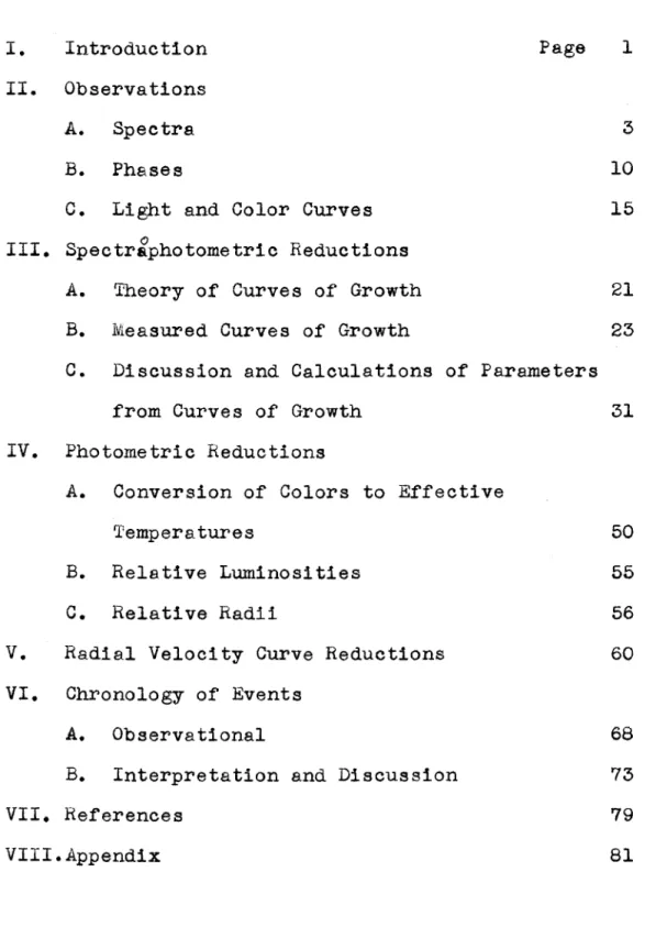
A. Conversion of Colors to Effective Temperatures In converting from colors, CP' to effective temperatures, Te, it would be convenient to use the six- color photometryof 238 stars by Stebbins and Whitfordl9.

First, the CP (photoelectric) color scale was founct²⁰ to coincide with the international color scale, Cint• The internationak color scale is based on the colors of nine 1

North Polar Sequence stars21. Stebbins and Whitfordl9 give Cint and the broad base line color V-I (violet minus infra red colors for ~eff

=

⁴²²⁰

i,

^10,300

i}

for these nine stars plus others. A least squares solution straight line gives:

v - I

= -

^1.582

±

^{o.157 +} _{2.744 c 1}^{nt (20}}

The values of V - I are listed in Table 10 for the color curve of Fig. 5 • Then using their relation between V - I and spectral clasal9, the spectral classes given in Table 10 have been derived.

To convert from colors V-I to temperatures we must choose between Stebbins and Whitford's T1 and T2 scales. The T1 scale is based on T1

=

6000° for dGO; for dG2 like the sun, T1

=

^5800°. The T2 scale is based on T2

=

6700° for dG2. Since the effective temperature of the sun is 5713°

and the color temperature, T₀, is 6500°, it appears that the

'1'2 scale is much closer to the Tc scale f'or stars of tempera-

- 50 -

tures near to the sun. This relation, T2

=

Tc, will be incorrect for early type stars. So in Table 10 we convert from V-I to T₀

=

^T2, using the data in columns 2 and 3 of

Table 11 which were taken from Stebbins and Whitford's paperl9. Next, to convert.Tc to effective temperatures,

Te

=

⁵

o

⁴

o ,

we will use the { Sc, ee) relation derived

by

Be

Chandrasekhar and Milnchl6, taking into consideration H- opacity. In Table 5 and Fig. 2 of their paper they relate

Phase

.oo

.05 .10 .15 .20 .25 .30 .35

~40

.45 .50 .55 .60 .65 .70 .75 .80 .85 .90 .95 1.00

cP

.34 .42 .48 .54 .60 .66

• 72 .78 .85 .90 .96 1.00

• 98 .93 .86 .78 .66 .50 .29 .27 .34

Table 10

Errective Temperatures V-I

- .65 - • 53 - • 26 - .10 .07 .23 .40 .56 .75 .89 1.06 1.17 1.11 .97 .78 .56 .23 - .21 - .78 - .84 - .65

Sp.

F4 F5 cF7 cF7.5 cF8 cGO cGl cG2 cG3 cG4 cG5 cG6 cG6 cG4.5 cG3.5 cG2 cGO cF7

F3

F2

F4

T2=Tc 8040 7650 6860 6480 6150 5890 5630 5400 5140 4970 4770 4660 4720 4870 5100 5400 5890 6750 8500 8720 8040

ec

.627 .659 .734 .777 .819 .856 .895 .933 .980 1.012 1.055 1.080 1.067 1.034 .988 .933 .856 .747 .593

• 578 .627

Se

.760 .773 .843 .881 .923 .966 1.020 1.075 1.157 1.190 1.253 1.290 1.270 1.242 1.155 1.075 .966 .855 .737 .726 .760

Table 11 Conversions of Colors

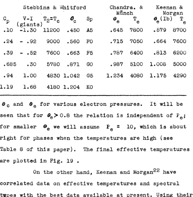
Stebbins & Whitford Chandra.. & Keenan &

ivlllnch Morgan Gp V-I T2:'11c ec Sp ee ^T ee (Ib) T

(giants) e e

.10 -1.30 11200 .450 A5 .645 7800 .579 8700 .24

-

^{.92 9000 .560 FO} .715 7050 .664 7600 .39

-

^{.52 '7600 .663 F5 .787 6400} .813 6200 .685 .30 5780 .871 GO .987 5100 1.008 5000 .94 1.00 4830 1.042 G5 1.234 4080 1.175 4290 1.19 1.68 4180 1.204 KO

6 ₀ and

ee

for various electron pressures. It will be seen that for Be> 0.8 the relation is independent of Pe;

for smaller Se we will assume ~e

=

10, which is about right for phases when the temperatures are high (see

Table 8 of this paper). The final effective temperatures are plotted in Fig. 19 •

On the other hand, Keenan and Morgan22 have correlated data on effective temperatures and spectral

t~pes with the best data available at present. Using their (spectral type, Te) correlation, we obtain the effective

temperatures in the last column of Table 11 from the spectral types in the fifth column. In the range from F2 to G6 the agreement between the empirical Keenan and Morgan and the theoretical Chandrasekhar and M-linch effective temperatures is good to within 200°, which is adequate. The probable

- 52 -

error of

±

01Po2 in the colors, CP' corresponds to a probable error of about 100° in the temperatures. The probable error in the excitation temperatures for FeI is

about 150 to 300°. The spectral classes from the colors agree to within one or two tenths of a class with Eggen's correlation23 of

cP

with spectral class for stars of

luminosity class Ib.

- 54 -

B. Relative Luminosities

Using the spectral types derived from the colors (Table 10}, we can obtain empirical bolometric corrections from G.P. Kuiper's paper24. Table 12 gives the following:

m5000 (Gordon-Kron light curve with m4260 at maximum= ^9.9};

Cp (Fig. 5),·

m

₅₄₅

o ( = m

5450-5000 C : photovisual 5000 - 5280-4260 p

magnitude); bolometric correction, B.C.; and, mbol• Then from the apparant bolometric magnitudes, e. lnnol~ we can obtain relative luminosities from

- 5 l L IDmin - m - - og - '

2 L.min (21)

where the subscripts refer to minimum photographic light.

Phase

.oo

.05 .10 .15 .20 .25 .30 .35 .40 .45

• 50 .55 .60 .65 .70 .75 .80

'I'able 12

Relative Luminosities and Radii m5000

9.70 9.74 9.78 9.80 9.85 9.89 9.94 10.01 10.17 10.41 10.66 10.90 11.07 11.06 10.88 10.70 10.49

cP

.34 .42 .48 .54 .60 .66 .72 .78 .85 .90 .96 1.00 .98 .93 .86 .78 .66

m5450 9.55 9.55 9.57 9.56 9.59 9.60 9.62 9.67 9.80 10.01 10.24 10.46 10.64 10.65 10.50 10.36 10.20

B.C.

- .07 - .11 - .22 - .25 - .28 - .42 - .48 - .52 - .57 - .60 - .65 - .69 - .69 - .63 - • 59 - .52 - .42

mbol 9.48 9.44 9.35 9.31 9.31 9.18 9.14 9.15 9.23 9.41 9.59 9.77 9.95 10.02 9.91 9.84 9.78'

L/Lmin 1.644 1.706 1.854 1.923 1.923 2.168 2.249 2.228 2.070 1.754 1.486 1.259 1.067 1.000 1.107 1.180 1.247

R/R max .384 .404 .502 .558 .613 .712 .809 .893 1.000 .972 .992 .968 .863 .801 .727 .650 .540