Advanced Modelling in Finance
using Excel and VBA
Wiley Finance Series
Operational Risk: Measurement and Modelling Jack King
Advance Credit Risk Analysis: Financial Approaches and Mathematical Models to Assess, Price and Manage Credit Risk
Didier Cossin and Hugues Pirotte Dictionary of Financial Engineering
John F. Marshall
Pricing Financial Derivatives: The Finite Difference Method Domingo A Tavella and Curt Randall
Interest Rate Modelling
Jessica James and Nick Webber
Handbook of Hybrid Instruments: Convertible Bonds, Preferred Shares, Lyons, ELKS, DECS and Other Mandatory Convertible Notes
Izzy Nelken (ed)
Options on Foreign Exchange, Revised Edition David F DeRosa
The Handbook of Equity Derivatives, Revised Edition Jack Francis, William Toy and J Gregg Whittaker
Volatility and Correlation in the Pricing of Equity, FX and Interest-Rate Options Riccardo Rebonato
Risk Management and Analysis vol. 1: Measuring and Modelling Financial Risk Carol Alexander (ed)
Risk Management and Analysis vol. 2: New Markets and Products Carol Alexander (ed)
Implementing Value at Risk Philip Best
Credit Derivatives: A Guide to Instruments and Applications Janet Tavakoli
Implementing Derivatives Models Les Clewlow and Chris Strickland
Interest-Rate Option Models: Understanding, Analysing and Using Models for Exotic Interest-Rate Options (second edition)
Riccardo Rebonato
Advanced Modelling in Finance using Excel and VBA
Mary Jackson and
Mike Staunton
JOHN WILEY & SONS, LTD
ChichesteržNew Yorkž WeinheimžBrisbanež Singaporež Toronto
Copyright2001 by John Wiley & Sons, Ltd, Baffins Lane, Chichester, West Sussex PO19 1UD, England National 01243 779777 International (C44) 1243 779777
e-mail (for orders and customer service enquiries): [email protected] Visit our Home Page on http://www.wiley.co.uk
or http://www.wiley.com
All Rights Reserved. No part of this publication may be reproduced, stored in a retrieval system, or transmitted, in any form or by any means, electronic, mechanical, photocopying, recording, scanning or otherwise, except under the terms of the Copyright, Designs and Patents Act 1988 or under the terms of a licence issued by the Copyright Licensing Agency, 90 Tottenham Court Road, London W1P 9HE, UK, without the permission in writing of the publisher.
Other Wiley Editorial Offices
John Wiley & Sons, Inc., 605 Third Avenue, New York, NY 10158-0012, USA
Wiley-VCH Verlag GmbH, Pappelallee 3, D-69469 Weinheim, Germany
John Wiley & Sons Australia Ltd, 42 McDougall Street, Milton, Queensland 4064, Australia
John Wiley & Sons (Asia) Pte Ltd, 2 Clementi Loop #02-01, Jin Xing Distripark, Singapore 129809
John Wiley & Sons Canada Ltd, 6045 Freemont Blvd, Mississauga, ONT, L5R 4J3, Canada
British Library Cataloguing in Publication Data
A catalogue record for this book is available from the British Library ISBN 0 471 49922 6
Typeset in 10/12pt Times by Laserwords Private Limited, Chennai, India Printed and bound in Great Britain by Bookcraft (Bath) Ltd, Midsomer–Norton
This book is printed on acid-free paper responsibly manufactured from sustainable forestry, in which at least two trees are planted for each one used for paper production.
Contents
Preface xi
Acknowledgements xii
1 Introduction 1
1.1 Finance insights 1
1.2 Asset price assumptions 2
1.3 Mathematical and statistical problems 2
1.4 Numerical methods 2
1.5 Excel solutions 3
1.6 Topics covered 3
1.7 Related Excel workbooks 5
1.8 Comments and suggestions 5
Part One Advanced Modelling in Excel 7
2 Advanced Excel functions and procedures 9
2.1 Accessing functions in Excel 9
2.2 Mathematical functions 10
2.3 Statistical functions 12
2.3.1 Using the frequency function 12
2.3.2 Using the quartile function 14
2.3.3 Using Excel’s normal functions 15
2.4 Lookup functions 16
2.5 Other functions 18
2.6 Auditing tools 19
2.7 Data Tables 20
2.7.1 Setting up Data Tables with one input 20
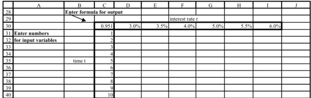
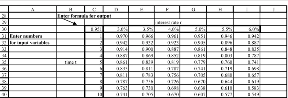
2.7.2 Setting up Data Tables with two inputs 22
2.8 XY charts 23
2.9 Access to Data Analysis and Solver 26
2.10 Using range names 27
2.11 Regression 28
2.12 Goal Seek 31
2.13 Matrix algebra and related functions 33
2.13.1 Introduction to matrices 33
2.13.2 Transposing a matrix 33
2.13.3 Adding matrices 34
2.13.4 Multiplying matrices 34
2.13.5 Matrix inversion 35
2.13.6 Solving systems of simultaneous linear equations 36
2.13.7 Summary of Excel’s matrix functions 37
Summary 37
3 Introduction to VBA 39
3.1 Advantages of mastering VBA 39
3.2 Object-oriented aspects of VBA 40
3.3 Starting to write VBA macros 42
3.3.1 Some simple examples of VBA subroutines 42
3.3.2 MsgBox for interaction 43
3.3.3 The writing environment 44
3.3.4 Entering code and executing macros 44
3.3.5 Recording keystrokes and editing code 45
3.4 Elements of programming 47
3.4.1 Variables and data types 48
3.4.2 VBA array variables 48
3.4.3 Control structures 50
3.4.4 Control of repeating procedures 51
3.4.5 Using Excel functions and VBA functions in code 52
3.4.6 General points on programming 53
3.5 Communicating between macros and the spreadsheet 53
3.6 Subroutine examples 56
3.6.1 Charts 56
3.6.2 Normal probability plot 59
3.6.3 Generating the efficient frontier with Solver 61
Summary 65
References 65
Appendix 3A The Visual Basic Editor 65
Stepping through a macro and using other
debug tools 68
Appendix 3B Recording keystrokes in ‘relative references’ mode 69
4 Writing VBA user-defined functions 73
4.1 A simple sales commission function 73
4.2 Creating Commission(Sales) in the spreadsheet 74
4.3 Two functions with multiple inputs for valuing options 75
4.4 Manipulating arrays in VBA 78
4.5 Expected value and variance functions with array inputs 79
4.6 Portfolio variance function with array inputs 81
4.7 Functions with array output 84
4.8 Using Excel and VBA functions in user-defined functions 85
Contents vii 4.8.1 Using VBA functions in user-defined functions 85
4.8.2 Add-ins 86
4.9 Pros and cons of developing VBA functions 86
Summary 87
Appendix 4A Functions illustrating array handling 88 Appendix 4B Binomial tree option valuation functions 89
Exercises on writing functions 94
Solution notes for exercises on functions 95
Part Two Equities 99
5 Introduction to equities 101
6 Portfolio optimisation 103
6.1 Portfolio mean and variance 103
6.2 Risk–return representation of portfolios 105
6.3 Using Solver to find efficient points 106
6.4 Generating the efficient frontier (Huang and Litzenberger’s
approach) 109
6.5 Constrained frontier portfolios 111
6.6 Combining risk-free and risky assets 113
6.7 Problem One–combining a risk-free asset with a risky asset 114
6.8 Problem Two–combining two risky assets 115
6.9 Problem Three–combining a risk-free asset with a risky portfolio 117
6.10 User-defined functions in Module1 119
6.11 Functions for the three generic portfolio problems in Module1 120
6.12 Macros in ModuleM 121
Summary 123
References 123
7 Asset pricing 125
7.1 The single-index model 125
7.2 Estimating beta coefficients 126
7.3 The capital asset pricing model 129
7.4 Variance–covariance matrices 130
7.5 Value-at-Risk 131
7.6 Horizon wealth 134
7.7 Moments of related distributions such as normal and lognormal 136
7.8 User-defined functions in Module1 136
Summary 138
References 138
8 Performance measurement and attribution 139
8.1 Conventional performance measurement 140
8.2 Active–passive management 141
8.3 Introduction to style analysis 144
8.4 Simple style analysis 145
8.5 Rolling-period style analysis 146
8.6 Confidence intervals for style weights 148
8.7 User-defined functions in Module1 151
8.8 Macros in ModuleM 151
Summary 152
References 153
Part Three Options on Equities 155
9 Introduction to options on equities 157
9.1 The genesis of the Black–Scholes formula 158
9.2 The Black–Scholes formula 158
9.3 Hedge portfolios 159
9.4 Risk-neutral valuation 161
9.5 A simple one-step binomial tree with risk-neutral valuation 162
9.6 Put–call parity 163
9.7 Dividends 163
9.8 American features 164
9.9 Numerical methods 164
9.10 Volatility and non-normal share returns 165
Summary 165
References 166
10 Binomial trees 167
10.1 Introduction to binomial trees 167
10.2 A simplified binomial tree 168
10.3 The Jarrow and Rudd binomial tree 170
10.4 The Cox, Ross and Rubinstein tree 173
10.5 Binomial approximations and Black–Scholes formula 175
10.6 Convergence of CRR binomial trees 176
10.7 The Leisen and Reimer tree 177
10.8 Comparison of CRR and LR trees 178
10.9 American options and the CRR American tree 180
10.10 User-defined functions in Module0 and Module1 182
Summary 183
References 184
11 The Black–Scholes formula 185
11.1 The Black–Scholes formula 185
11.2 Black–Scholes formula in the spreadsheet 186
11.3 Options on currencies and commodities 187
11.4 Calculating the option’s ‘greek’ parameters 189
11.5 Hedge portfolios 190
11.6 Formal derivation of the Black–Scholes formula 192
Contents ix
11.7 User-defined functions in Module1 194
Summary 195
References 196
12 Other numerical methods for European options 197
12.1 Introduction to Monte Carlo simulation 197
12.2 Simulation with antithetic variables 199
12.3 Simulation with quasi-random sampling 200
12.4 Comparing simulation methods 202
12.5 Calculating greeks in Monte Carlo simulation 203
12.6 Numerical integration 203
12.7 User-defined functions in Module1 205
Summary 207
References 207
13 Non-normal distributions and implied volatility 209 13.1 Black–Scholes using alternative distributional assumptions 209
13.2 Implied volatility 211
13.3 Adapting for skewness and kurtosis 212
13.4 The volatility smile 215
13.5 User-defined functions in Module1 217
Summary 219
References 220
Part Four Options on Bonds 221
14 Introduction to valuing options on bonds 223
14.1 The term structure of interest rates 224
14.2 Cash flows for coupon bonds and yield to maturity 225
14.3 Binomial trees 226
14.4 Black’s bond option valuation formula 227
14.5 Duration and convexity 228
14.6 Notation 230
Summary 230
References 230
15 Interest rate models 231
15.1 Vasicek’s term structure model 231
15.2 Valuing European options on zero-coupon bonds, Vasicek’s model 234 15.3 Valuing European options on coupon bonds, Vasicek’s model 235
15.4 CIR term structure model 236
15.5 Valuing European options on zero-coupon bonds, CIR model 237 15.6 Valuing European options on coupon bonds, CIR model 238
15.7 User-defined functions in Module1 239
Summary 240
References 241
16 Matching the term structure 243 16.1 Trees with lognormally distributed interest rates 243
16.2 Trees with normal interest rates 246
16.3 The Black, Derman and Toy tree 247
16.4 Valuing bond options using BDT trees 248
16.5 User-defined functions in Module1 250
Summary 252
References 252
Appendix Other VBA functions 253
Forecasting 253
ARIMA modelling 254
Splines 256
Eigenvalues and eigenvectors 257
References 258
Index 259
Preface
When asked why they tackled Mount Everest, climbers typically reply “Because it was there”. Our motivation for writing Advanced Modelling in Finance is for exactly the opposite reason. There were then, and still are now, almost no books that give due prominence to and explanation of the use of VBA functions within Excel. There is an almost similar lack of books that capture the true vibrant spirit of numerical methods in finance.
It is no longer true that spreadsheets such as Excel are inadequate tools in highly tech- nical and numerically demanding areas such as the valuation of financial derivatives. With efficient code and VBA functions, calculations that were once the preserve of dedicated packages and languages can now be done on a modern PC in Excel within seconds, if not fractions of a second. By employing Excel and VBA, our purpose is to try to bring clarity to an area that was previously covered with black boxes.
What started as an attempt to push back the boundaries of Excel through macros turned into a full-scale expedition into the VBA language within Excel and then developed from equities, through options and finally to cover bonds. Along the way we learned scores of new Excel skills and a much greater understanding of the numerical methods implemented across finance.
The genesis of the book came from material developed for the ‘Computer-Based Finan- cial Modelling’ elective on the MBA degree at London Business School. The part on equities formed the basis for an executive course on ‘Equity Portfolio Management’ run annually by the International Centre for Money and Banking in Geneva. The parts on options and bonds comprise a course in ‘Numerical Methods’ on the MSc in Mathemat- ical Trading and Finance at City University Business School. The book is within the reach of both students at the postgraduate level and those in the latter undergraduate years.
There are no prerequisites for readers apart from a willingness to adopt a pro-active stance when using the book–namely by taking advantage of the inherent ‘what-if’ quality of the spreadsheets and by looking at and using the code forming the VBA user-defined functions. Since we assume for the most part that asset returns are lognormal and therefore use binomial trees as a central numerical method, our explanations can be based on familiar results from probability and statistics. Comprehension is helped by the use of a common notation throughout, and transparency by the availability of complete solutions in both Excel and VBA forms.
Acknowledgements
Our main debt is to the individuals from the academic and practitioner communities in finance who first developed the theory and then the numerical methods that form the material for this book. In the words of Sir Isaac Newton “If I have seen further it is by standing on the shoulders of giants”.
We would also like to thank our colleagues at both London Business School and City University Business School, in particular Elroy Dimson, John Hatgioannides, Paul Marsh and Kiriakos Vlahos.
We would like to thank Sam Whittaker at Wiley for her enthusiasm, encouragement and much needed patience, invaluable qualities for an editor.
Last but not least, we are grateful for the patience of family and friends who have occasionally chivvied us about the book’s somewhat lengthy gestation period.
1
Introduction
We hope that our text, Advanced Modelling in Finance, is conclusive proof that a wide range of models can now be successfully implemented using spreadsheets. The models range across the complete spectrum of finance including equities, equity options and bond options spanning developments from the early fifties to the late nineties. The models are implemented in Excel spreadsheets, complemented with functions written using the VBA language within Excel. The resulting user-defined functions provide a portable library of programs with more than sufficient speed and accuracy.
Advanced Modelling in Finance should be viewed as a complement (or dare we say, an antidote) to traditional textbooks in the area. It contains relatively few derivations, allowing us to cover a broader range of models and methods, with particular emphasis on more recent advances.
The major theoretical developments in finance such as portfolio theory in the 1950s, the capital asset pricing model in the 1960s and the Black–Scholes formula in the 1970s brought with them analytic solutions that are now straightforward to calculate. The subse- quent decades have seen a growing body of developments in numerical methods. With an intelligent choice of parameters, binomial trees have assumed a central role in the more numerically-intensive calculations now required to value equity and bond options. The centre of gravity in finance now concerns the search for more efficient ways of performing such calculations rather than the theories from yesteryear.
The breadth of the coverage across finance and the sophistication needed for some of the more advanced models are testament to the ability of Excel, the built-in functions contained in Excel and the real programming environment that VBA provides. This allows us to highlight the commonality of assumptions (lognormality), mathematical problems (expectation) and numerical methods (binomial trees) throughout finance as a whole.
Without exception, we have tried to ensure a consistent and simple notation throughout the book to reinforce this commonality and to improve clarity of exposition.
Our objective in writing a book that covers the broad range of subjects in finance has proved to be both a challenge and an opportunity. The opportunity has provided us with the chance to overview finance as a whole and, in so doing, to make impor- tant connections and bring out commonalities in asset price assumptions, mathemat- ical problems, numerical methods and Excel solutions. In the following sections we summarise a few of these unifying insights that apply to equities, options and bonds with regard to finance, mathematical topics, numerical methods and Excel features. This is followed by a more detailed summary of the main topics covered in each chapter of the book.
1.1 FINANCE INSIGHTS
The genesis of modern finance as a subject separate from economics started with Markowitz’s development of portfolio theory in 1952. Markowitz used utility theory to model the preferences of individual investors and to develop a mean–variance approach
to examining the trade-off between return (as measured by an asset’s mean return) and risk (measured by an asset’s variance of return). This subsequently led to the development by Sharpe, Lintner and Treynor of the capital asset pricing model (CAPM), an equilibrium model describing expected returns on equities. The CAPM introduced beta as a measure of diversifiable risk, arguing that the creation of portfolios served to minimise the specific risk element of total risk (variance).
The next great theoretical development was the equity option pricing formula of Black and Scholes, which rested on the ability to create a (riskless) hedge portfolio. Contempora- neously, Merton extended the Black–Scholes formula to allow for continuous dividends and thus also options on commodities and currencies. The derivation of the original formula required the solving of the diffusion (or heat) equation familiar from physics, but was subsequently encompassed by the broader risk-neutral approach to the valuation of derivatives.
1.2 ASSET PRICE ASSUMPTIONS
Although portfolio theory was derived through individual preferences, it could also have been obtained by making assumptions about the distribution of asset price returns. The standard assumption is that equity returns follow a lognormal distribution–equivalently we can say that equity log returns follow a normal distribution. More recently, practitioners have examined the effect of departures from strict normality (as measured by skewness and kurtosis) and have also proposed different distributions (for example, the reciprocal gamma distribution).
Although bonds have characteristics that are different from equities, the starting point for bond option valuation is the short interest rate. This is frequently assumed to follow the lognormal or normal distribution. The result is that familiar results grounded in these probability distributions can be applied throughout finance.
1.3 MATHEMATICAL AND STATISTICAL PROBLEMS
Within the equities part, the mathematical problems concern optimisation. The optimi- sation can also include additional constraints, exemplified by Sharpe’s development of returns-based style analysis. Beta is estimated as the slope coefficient in a linear regression.
Options are valued in the risk-neutral framework as statistical expectations. The normal distribution of log equity prices can be approximated by an equivalent discrete bino- mial distribution. This binomial distribution provides the framework for calculating the expected option value.
1.4 NUMERICAL METHODS
In the context of portfolio optimisation, the optimisation involves portfolio variance, and the numerical method needed for optimisation is quadratic programming. Style analysis also uses quadratic programming, the quantity to be minimised being the error variance.
Although not usually thought of as optimisation, linear regression chooses slope coef- ficients to minimise residual error. Here optimisation is of a different kind, regression analysis, which provides analytical formulas to calculate the beta coefficients.
Turning to option valuation, the binomial tree provides the structure within which the risk-neutral expectation can be calculated. We highlight the importance of parameter
Introduction 3 choice by examining the convergence properties of three different binomial trees. Such trees also allow the valuation of American options, where the option can be exercised at any date prior to maturity.
With European options, techniques such as Monte Carlo simulation and numerical integration are also used. Numerical search methods, in particular the Newton–Raphson approach, ensure that volatilities implied by option prices in the market can be estimated.
1.5 EXCEL SOLUTIONS
The spreadsheets demonstrate how Excel can be used as a prototype for building models.
Within the individual spreadsheets, all the formulas in the cells can easily be examined and we have endeavoured to incorporate all intermediate calculations in cells of their own. The spreadsheets also allow the hallmark ability to ‘what-if’ by changing parameter values in cells.
The implementation of all the models and methods occurs twice: once in the spread- sheets and once in the VBA functions. This dual approach serves as an important check on the accuracy of the numerical calculations.
Some of the VBA procedures are macros, normally seen by others as the main purpose of VBA in Excel. However, the majority of the procedures we implement are user-defined functions. We demonstrate how easily these functions can be written in VBA and how they can incorporate Excel functions, including the powerful matrix functions.
The Goal Seek and Solver commands within Excel are used in the optimisation tasks.
We show how these commands can be automated using VBA user-defined functions and macros. Another under-used aspect of Excel involves the application of array functions (invoked by the CtrlCShiftCEnter keystroke combination) and we implement these in user-defined functions. To improve efficiency, our binomial trees in user-defined functions use one-dimensional arrays (vectors) rather than two-dimensional arrays (matrices).
1.6 TOPICS COVERED
There are four parts in the book, the first part illustrating the advanced modelling features in Excel followed by three parts with applications in finance. The three parts on applica- tions cover equities, options on equities and options on bonds.
Chapter 2 emphasises the advanced Excel functions and techniques that we use in the remainder of the book. We pay particular attention to the array functions within Excel and provide a short section detailing the mathematics underlying matrix manipulation.
Chapter 3 introduces the VBA programming environment and illustrates a step-by-step approach to the writing of VBA subroutines (macros). The examples chosen demonstrate how macros can be used to automate and repeat tasks in Excel.
Chapter 4 moves on to VBA user-defined functions, which have a crucial role throughout the applications in finance. We emphasise how to deal with both scalar and array variables–as input variables to VBA functions, their use in calculations and finally as output variables. Again, we use a step-by-step approach for a number of examples. In particular, we write user-defined functions to value both European options (the Black–Scholes formula) and American options (binomial trees).
Chapter 5 introduces the first application part, that dealing with equities.
Chapter 6 covers portfolio optimisation, using both Solver and analytic solutions. As will become the norm in the remaining chapters, Solver is used both in the spreadsheet
and automated in a VBA macro. By using the array functions in Excel and VBA, we detail how the points on the efficient frontier can be generated. The development of portfolio theory is divided into three generic problems, which recur in subsequent chapters.
Chapter 7 looks at (equity) asset pricing, starting with the single-index model and the capital asset pricing model (CAPM) and concluding with Value-at-Risk (VaR). This introduces the assumption that asset log returns follow a normal distribution, another recurrent theme.
Chapter 8 covers performance measurement, again ranging from single-parameter measures used in the very earliest days to multi-index models (such as style analysis) that represent current best practice. We show, for the first time in a textbook, how confidence intervals can be determined for the asset weights from style analysis.
Chapter 9 introduces the second application part, that dealing with options on equities.
Building on the normal distribution assumed for equity log returns, we detail the creation of the hedge portfolio that is the key insight behind the Black–Scholes option valuation formula. The subsequent interpretation of the option value as the discounted expected value of the option payoff in a risk-neutral world is also introduced.
Chapter 10 looks at binomial trees, which can be viewed as a discrete approxima- tion to the continuous normal distribution assumed for log equity prices. In practice, binomial trees form the backbone of numerical methods for option valuation since they can cope with early exercise and hence the valuation of American options. We illustrate three different parameter choices for binomial trees, including the little-known Leisen and Reimer tree that has vastly superior convergence and accuracy properties compared to the standard parameter choices. We use a nine-step tree in our spreadsheet examples, but the user-defined functions can cope with any number of steps.
Chapter 11 returns to the Black–Scholes formula and shows both its adaptability (allowing options on assets such as currencies and commodities to be valued) and its dependence on the asset price assumptions.
Chapter 12 covers two alternative ways of calculating the statistical expectation that lies behind the Black–Scholes formula for European options. These are Monte Carlo simulation and numerical integration. Although these perform less well for the simple options we consider, each of these methods has a valuable role in the valuation of more complicated options.
Chapter 13 moves away from the assumption of strict normality of asset log returns and shows how such deviation (typically through differing skewness and kurtosis parameters) leads to the so-called volatility smile seen in the market prices of options. Efficient methods for finding the implied volatility inherent in European option prices are described.
Chapter 14 introduces the third application part, that dealing with options on bonds.
While bond prices have characteristics that are different from equity prices, there is a lot of commonality in the mathematical problems and numerical methods used to value options. We define the term structure based on a series of zero-coupon bond prices, and show how the short-term interest rate can be modelled in a binomial tree as a means of valuing zero-coupon bond cash flows.
Chapter 15 covers two models for interest rates, those of Vasicek and Cox, and Ingersoll and Ross. We detail analytic solutions for zero-coupon bond prices and options on zero- coupon bonds together with an iterative approach to the valuation of options on coupon bonds.
Chapter 16 shows how the short rate can be modelled in a binomial tree in order to match a given term structure of zero-coupon bond prices. We build the popular
Introduction 5 Black–Derman–Toy interest rate tree (both in the spreadsheet and in user-defined func- tions) and show how it can be used to value both European and American options on zero-coupon bonds.
The final Appendix is a Pandora’s box of other user-defined functions, that are less rele- vant to the chosen applications in finance. Nevertheless they constitute a useful toolbox, including as they do functions for ARIMA modelling, splines, eigenvalues and other calculation procedures.
1.7 RELATED EXCEL WORKBOOKS
Part I which concentrates on Excel functions and procedures and understanding VBA has three related workbooks, AMFEXCEL, VBSUB and VBFNS which accompany Chap- ters 2, 3 and 4 respectively.
Part II on equities has three related workbooks, EQUITY1, EQUITY2 and EQUITY3 which accompany Chapters 6, 7 and 8 respectively.
Part III on options on equities has four files, OPTION1, OPTION2, OPTION3 and OPTION4 which accompany Chapters 10, 11, 12 and 13 respectively.
Part IV on bonds has two related workbooks, BOND1 and BOND2 which accompany Chapters 14, 15 and 16 as indicated in the text.
The Appendix has one workbook, OTHERFNS.
1.8 COMMENTS AND SUGGESTIONS
Having spent so much time developing the material and writing this book, we would very much appreciate any comments, suggestions and, dare we say, possible corrections and improvements. Please email [email protected] or find your way to www.london.edu/
ifa/services/services.html or www.business.city.ac.uk/irmi/mstaunton.html.
Part One
Advanced Modelling in Excel
2
Advanced Excel Functions and Procedures
The purpose of this chapter is to review certain Excel functions and procedures used in the text. These include mathematical, statistical and lookup functions from Excel’s extensive range of functions, as well as much-used procedures such as setting up Data Tables and displaying results in XY charts. Also included are methods of summarising data sets, conducting regression analyses, and accessing Excel’s Goal Seek and Solver.
The objective is to clarify and ensure that this material causes the reader no difficulty.
The advanced Excel user may wish to skim the content or use the chapter for further reference as and when required. To make the various topics more entertaining and more interactive, a workbook AMFEXCEL.xls includes the examples discussed in the text and allows the reader to check his or her proficiency.
2.1 ACCESSING FUNCTIONS IN EXCEL
Excel provides many worksheet functions, which are essentially calculation routines that have been coded up. They are useful for simplifying calculations performed in the spread- sheet, and also for combining into VBA macros and user-defined functions (topics covered in Chapters 3 and 4).
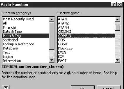
The Paste Function button (labelledfx) on the standard toolbar gives access to them. (It was previously known as the function wizard.) As Figure 2.1 shows, functions are grouped into different categories: mathematical, statistical, logical, lookup and reference, etc.
Figure 2.1 Paste Function dialog box showing the COMBIN function in the Math category
Here the Math & Trig function COMBIN has been selected, which produces a brief description of the function’s inputs and outputs. For a fuller description, press the Help button (labelled ?).
On clicking OK, the Formula palette appears providing slots for entering the appropriate inputs, as in Figure 2.2. The required inputs can be keyed into the slots (as here) or
‘selected’ by referencing cells in the spreadsheet (by clicking the buttons to collapse the Formula palette). Note that the palette can be dragged away from its standard position.
Clicking the OK button on the palette or the tick on the Edit line enters the formula in the spreadsheet.
Figure 2.2 Building the COMBIN function in the Formula palette
As well as the Formula palette with inputs for function COMBIN, Figure 2.2 shows the construction of the cell formula on the Edit line, with the Paste Function button depressed (in action). Notice also the Paste Name button (labelledDab) which facilitates pasting of named cells into the formula. (Attaching names to ranges and referencing cell ranges by names is reviewed in section 2.10.)
As well as all Excel functions, the Paste Function button also provides access to the user-defined category of functions which are described in Chapter 4.
Having discussed how to access the functions, in the following sections we describe some specific mathematical and statistical functions.
2.2 MATHEMATICAL FUNCTIONS
Within the Math & Trig category, we make use of the EXP(x), LN(x), SQRT(x), RAND(), FACT(x) and COMBIN(number, numberchosen) functions.
EXP(x) returns values of the exponential function, exp(x) or ex. For example:
ž EXP(1) returns value of e (2.7183 when formatted to four decimal places) ž EXP(2) returns value of e2 (7.3891 to four decimal places)
ž EXP(1) returns value of 1/e or e1 (0.36788 to five decimal places)
Advanced Excel Functions and Procedures 11 In finance calculations, cash flows occurring at different time periods are converted into future (or present) values by applying compounding (or discounting) factors. With continu- ous compounding at rate r, the compounding factor for one year is exp(r), and the equivalent annual interest ratera, if compounding were done on an annual basis, is given by the expression:
raDexpr1
Continuous compounding and the use of the EXP function is illustrated further in section 2.7.1 on Data Tables.
LN(x) returns the natural logarithm of valuex. Note thatxmust be positive, otherwise the function returns #NUM! for numeric overflow. For example:
ž LN(0.36788) returns value1 ž LN(2.7183) returns value 1 ž LN(7.3891) returns value 2 ž LN(4) returns value #NUM!
In finance, we frequently work with (natural) log returns, applying the LN function to transform the returns data into log returns.
SQRT(x) returns the square root of value x. Clearly,xmust be positive, otherwise the function returns #NUM! for numeric overflow.
RAND() generates a uniformly distributed random number greater than or equal to zero and less than one. It changes each time the spreadsheet recalculates. We can use RAND() to introduce probabilistic variability into Monte Carlo simulation of option values.
FACT(number) returns the factorial of the number, which equals 1Ł2Ł3Ł. . .Łnumber.
For example:
ž FACT(6) returns the value 720
COMBIN(number, numberchosen) returns the number of combinations (subsets of size ‘numberchosen’) that can be made up from a ‘number’ of items. The subsets can be in any internal order. For example, if a share moves either ‘up’ or ‘down’ at four discrete times, the number of sequences with three ups (and one down) is:
COMBIN4,1D4 or equally COMBIN4,3D4
that is the four sequences ‘up-up-up-down’, ‘up-up-down-up’, ‘up-down-up-up’ and
‘down-up-up-up’. In statistical parlance, COMBIN4,3is the number of combinations of three items selected from four and is usually denoted as4C3 (or in general,nCr).
Excel has functions to transpose matrices, to multiply matrices and to invert square matrices. The relevant functions are:
ž TRANSPOSE(array) which returns the transpose of an array
ž MMULT(array1, array2) which returns the matrix product of two arrays ž MINVERSE(array) which returns the matrix inverse of an array
These fall in the same Math category. Since some readers may need an introduction to matrices before examining the functions, this material has been placed at the end of the chapter (see section 2.13).
2.3 STATISTICAL FUNCTIONS
Excel has several individual functions for quickly summarising the features of a data set (an ‘array’ in Excel terminology). These include AVERAGE(array) which returns the mean, STDEV(array) for the standard deviation, MAX(array) and MIN(array) which we assume are familiar to the reader.
To obtain the distribution of a moderate sized data set, there are some useful functions that deserve to be better known. For example, the QUARTILE function produces the indi- vidual quartile values on the basis of the percentiles of the data set and the FREQUENCY function returns the whole frequency distribution of the data set after grouping.
Excel also provides functions for a range of different theoretical probability distri- butions, in particular those for the normal distribution: NORMSDIST and NORMSINV for the standard normal with zero mean and standard deviation one; NORMDIST and NORMINV for any normal distribution.
Other useful functions in the statistical category are those for two variables, which provide many individual quantities used in regression and correlation analysis. For example:
ž INTERCEPT(knowny’s, knownx’s) ž SLOPE(knowny’s, knownx’s) ž RSQ(knowny’s, knownx’s) ž STEYX(knowny’s, knownx’s) ž CORREL(array1, array2) ž COVAR(array1, array2)
There is also a little known array function, LINEST(knowny’s, knownx’s), which returns the essential regression statistics in array form. Most of these functions are exam- ined in more detail in section 2.11 on regression. Their performance is compared and contrasted with the regression output from the Data Analysis Regression procedure.
In the next section, we explain how to use the FREQUENCY, QUARTILE and various normal functions via examples in the Frequency and SNorm sheets of the AMFEXCEL workbook.
2.3.1 Using the Frequency Function
FREQUENCY(dataarray, binsarray) counts how often values in a data set occur within specified intervals (or ‘bins’), and then returns these frequencies in a vertical array. The binsarray is the set of intervals into which the values are grouped. Since the function returns output in the form of an array, it is necessary to mark out a range of cells in the spreadsheet to receive the outputbefore entering the function.
We explain how to use FREQUENCY with an example set out in the Frequency sheet of the AMFEXCEL workbook. As shown in Figure 2.3, monthly returns and log returns (using the LN function) in columns D10:D71 and E10:E70 have been summarised in rows 4 to 7. Suppose the aim is to get the frequency distribution of the log returns (E10:E71), i.e. the so-called ‘dataarray’. The objective might be to check that these returns are approximately normally distributed. First, we have to decide on intervals (or bins) for grouping the data. Inspection of the maximum and minimum log returns suggests about 10 to 12 intervals in the range0.16 toC0.20. The ‘interval’ values, which have
Advanced Excel Functions and Procedures 13 been entered in range G5:G14, act as upper limits when the log returns are grouped into the so-called ‘bins’.
2 3 4 5 6 7 8 9 10 11 12 13 14 15 16 17 18
A B C D E F G H I J
Returns for months 1 - 62
Summary Statistics: Returns Ln Returns Frequency Distribution:
Mean 1.78% 0.014 interval freq %freq %cum freq
St Dev 8.09% 0.080 -0.16
Max 21.23% 0.193 -0.12
Min -14.21% -0.153 -0.08
-0.04
Month Returns Ln Returns 0.00
Feb-92 1 7.06% 0.0682 0.04
Mar-92 2 -11.54% -0.1226 0.08
Apr-92 3 7.77% 0.0748 0.12
May-92 4 10.66% 0.1013 0.16
Jun-92 5 -11.72% -0.1247 0.20
Jul-92 6 -8.26% -0.0862
Aug-92 7 -2.89% -0.0293
Sep-92 8 9.93% 0.0947 Total
Oct-92 9 12.65% 0.1191
Figure 2.3 Layout for calculating the frequency distribution of log returns data
To enter the FREQUENCY function correctly, select the range H5:H15. Then start by typingDand clicking on the Paste Function button (labelledfx) to complete the function syntax:
=FREQUENCY(E10:E71,G5:G14)
After adding the last bracket ‘)’, with the cursor on Excel’s Edit line, enter the function by holding down the Ctrl then the Shiftthen the Enter keys. (You need to use three fingers, otherwise it will not work. If this fails, keep the output range of cells ‘selected’, press the Edit key (F2), edit the formula if necessary, then press CtrlCShiftCEnter once again.)
You should now see the function enclosed in curly brackets fg in the cells, and the frequencies array in cells G5:G15. The results are in Figure 2.4. Use the SUM function in cell H17 to check that the frequencies sum to 62.
Interpreting the results, we can see that there were no log returns below0.16, six values in the range 0.16 to0.12 and no values above 0.20. (The bottom cell in the FREQUENCY array, G15, contains any values above the bins’ upper limit, 0.20.)
Since the FREQUENCY function has array output, individual cells cannot be changed.
If a different number of intervals is required, the current array must be deleted and the function entered again.
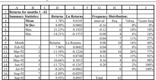
It helps to convert the frequencies into percentage frequencies (relative to the size of the data set of 62 values) and then to calculate cumulated percentage frequencies as shown in columns I and J in Figure 2.4. The percentage frequency and cumulative percentage frequency formulas can be examined in the Frequency sheet.
2 3 4 5 6 7 8 9 10 11 12 13 14 15 16 17
A B C D E F G H I J
Returns for months 1 - 62
Summary Statistics: Returns Ln Returns Frequency Distribution:
Mean 1.78% 0.0145 interval freq %freq %cum freq
St Dev 8.09% 0.0802 -0.16 0 0% 0%
Max 21.23% 0.1925 -0.12 6 10% 10%
Min -14.21% -0.1533 -0.08 4 6% 16%
-0.04 7 11% 27%
Month Returns Ln Returns 0.00 10 16% 44%
Feb-92 1 7.06% 0.0682 0.04 5 8% 52%
Mar-92 2 -11.54% -0.1226 0.08 16 26% 77%
Apr-92 3 7.77% 0.0748 0.12 9 15% 92%
May-92 4 10.66% 0.1013 0.16 4 6% 98%
Jun-92 5 -11.72% -0.1247 0.20 1 2% 100%
Jul-92 6 -8.26% -0.0862 0 0% 100%
Aug-92 7 -2.89% -0.0293
Sep-92 8 9.93% 0.0947 Total 62
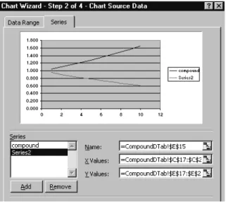
Figure 2.4 Frequency distribution of log returns with % frequency and cumulative distributions The best way to display the percentage cumulative frequencies is an XY chart with data points connected by a smooth line with no markers. To produce a chart like that in Figure 2.5, select ranges G5:G14 and J5:J14 as the source data. Note that, to select non-contiguous ranges, select the first range, then hold down the Ctrl key whilst selecting the second and subsequent ranges.
3 4 5 6 7 8 9 10 11 12 13 14 15 16 17
F G H I J K L M N O P Q R
Frequency Distribution:
interval freq %freq %cum freq theory
-0.16 0 0% 0% 1%
-0.12 6 10% 10% 5%
-0.08 4 6% 16% 12%
-0.04 7 11% 27% 25%
0.00 10 16% 44% 43%
0.04 5 8% 52% 62%
0.08 16 26% 77% 79%
0.12 9 15% 92% 91%
0.16 4 6% 98% 97%
0.20 1 2% 100% 99%
0 0% 100% 43%
Total 62
Cumulative Frequency
0%
25%
50%
75%
100%
-0.20 -0.10 0.00 0.10 0.20
ln(return) actual
theory
Figure 2.5 Chart of cumulative % frequencies (actual and strictly normal data)
For normally distributed log returns, the cumulative distribution should be sigmoid in shape (as indicated by the dashed line). The actual log returns data shows some departure from normality, possibly due to skewness.
2.3.2 Using the Quartile Function
QUARTILE(array, quart) returns the quartile of a data set. The second input ‘quart’ is an integer that determines which quartile is returned: if 0, the minimum value of the array;
if 1, the first quartile (i.e. the 25th percentile of the array); if 2, the median value (50th percentile); if 3, the third quartile (75th percentile); if 4, the maximum value.
Advanced Excel Functions and Procedures 15 The quartiles provide a quick and relatively easy way to get the cumulative distribution of a data set. For example in cell H22 in Figure 2.6, the entry:
QUARTILE(E10:E71,G22)
where G22 contains the integer value 1, returns the first quartile. The value displayed in the cell is 0.043, which is the log return value below which 25% of the values in the data set fall. The second quartile, 0.028, is the median and the third quartile, 0.075, is the value below which 75% of the values fall. Figure 2.6 also shows an XY chart of the range H21:I25 with the data points marked. The cumulative curve based on just five data points can be seen to be quite close to the more accurate version in Figure 2.5.
18 19 20 21 22 23 24 25 26 27 28 29
F G H I J K L M N O P Q
Quartiles:
quart no. Q points Q %
0 -0.153 0%
1 -0.043 25%
2 0.028 50%
3 0.075 75%
4 0.193 100%
Cumulative Frequency from quartiles
0%
25%
50%
75%
100%
-0.20 -0.10 0.00 0.10 0.20
ln(return)
Figure 2.6 Quartiles for the log returns data in the Frequency sheet
The QUARTILE function is used in section 3.5 to illustrate array handling in VBA. A related function, PERCENTILE(array, k) which returns the kth percentile of a data set, is used to illustrate coding an array function in section 4.7.
2.3.3 Using Excel’s Normal Functions
Of the statistical functions related to normal distribution, their names all start with the four letters NORM, and some include an S to indicate that the standard normal distribution is assumed.
NORMSDIST(z) returns the cumulative distribution function for the standard normal distribution. NORMSINV(probability) returns values of zfor specified probabilities.
The rather more versatile NORMDIST(x, mean, standarddev, cumulative) applies to any normal distribution. If the ‘cumulative’ input parameterD1 (or TRUE), it returns values for the cumulative distribution function; if ‘cumulative’ inputD0 (or FALSE), it returns the probability density function.
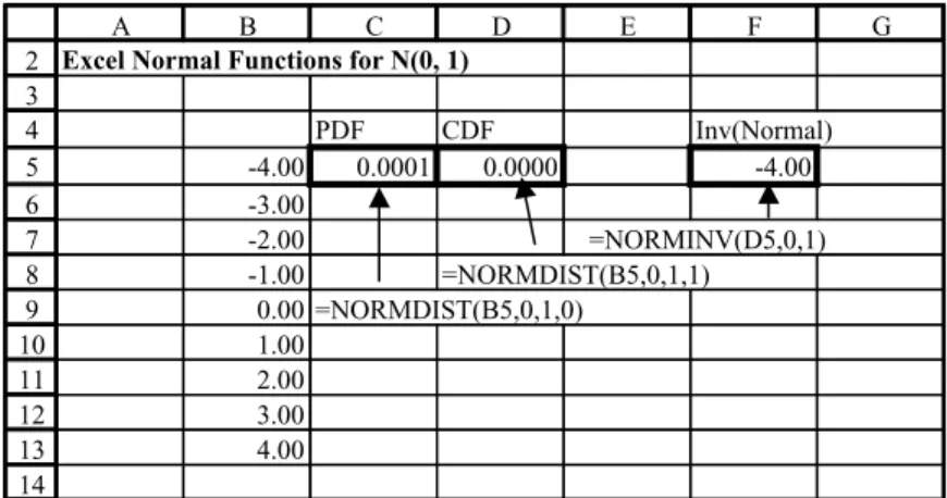
Figure 2.7 shows the Norm sheet, with entries for the probability density and for the left-hand tail probability in cells C5 and D5 respectively. Both these formulas use the general NORMDIST function with mean and standard deviation inputs set to 0 and 1 respectively. In C5, the last input (‘cumulative’) takes value 0 for the probability density and in D5 takes value 1 for the left-hand tail probability.
The ordinate values corresponding to left-hand tail probabilities can be obtained from the NORMINV function as shown in cell F5.
To familiarise yourself with these functions, copy the formulas down and examine the results.
In the last section, we obtained a cumulative percentage frequency distribution for log returns. One check on normality is to use the NORMDIST function with the observed mean and standard deviation to calculate theoretical percentage frequencies. This has been done in column K of the Frequency sheet. The resulting frequencies are shown in the Figure 2.5 chart, superimposed on the distribution of actual returns. Some departures from normality can be seen.
2 3 4 5 6 7 8 9 10 11 12 13 14
A B C D E F G
Excel Normal Functions for N(0, 1)
PDF CDF Inv(Normal)
-4.00 0.0001 0.0000 -4.00
-3.00
-2.00 =NORMINV(D5,0,1)
-1.00 =NORMDIST(B5,0,1,1) 0.00 =NORMDIST(B5,0,1,0)
1.00 2.00 3.00 4.00
Figure 2.7 Excel’s general normal distribution functions in the SNorm sheet
Excel provides an excellent range of functions for data summary, and for modelling various theoretical distributions. We make considerable use of them in both the Equity and the Options parts of the text.
2.4 LOOKUP FUNCTIONS
In tables of related information, ‘lookups’ allow items of information to be extracted on the basis of different lookup inputs. For example, in Figure 2.8 we illustrate the use of the VLOOKUP function which for a given volatility value ‘looks up’ the Black–Scholes call value from a table of volatilities and related call values. (We shall cover the background theory in Chapter 11 on the Black–Scholes formula.)
In general the function:
VLOOKUP(lookupvalue, tablearray, colindexnum, rangelookup)
searches for a value in the leftmost column of a table (tablearray), and then returns a value in the same row from a column you specify (with colindexnum). By default, the first column of the table must be in ascending order (which implies that rangelookupD1 (or TRUE)). In fact, if this is the case, the last input parameter can be ignored.
Lookup examples are in the LookUp sheet. To check your understanding, use the VLOOKUP function to decide the commission to be paid on different sales amounts, given the commission rates table in cell range F5:G7. Then scroll down to the Black–Scholes Call Value LookUp Table, illustrated in Figure 2.8.
The lookupvalue (for volatility) is in C17 (20%), the table array is F17:G27, with volatilities in ascending order and call values in column 2 of the table array. So the
Advanced Excel Functions and Procedures 17 formula in cell D18:
DVLOOKUP(C17,F17:G27,2) returns a call value of 9.73 for the 20% volatility.
15 16 17 18 19 20 21 22 23 24 25 26 27 28
A B C D E F G H
Black-Scholes Call Value Lookup Table
Volatility BS Call Value
Volatility 20% 15% 8.63
VLOOKUP 16% 8.84
17% 9.05
18% 9.27
call value 9.73 19% 9.50
MATCH 20% 9.73
21% 9.96
22% 10.19
row 6 23% 10.43
column 2 24% 10.67
INDEX 25% 10.91
Figure 2.8 Layout for looking up call values given volatility in the LookUp sheet
The lookupvalue is matched approximately (or exactly) against values in the first column of the table, a row selected on the basis of match and the entry in the specified column returned. Try experimenting with different volatility values such as 20.5%, 21.5% in cell C17 to see how the lookup function works.
The rangelookup input is a logical value (TRUE or FALSE) which specifies whether you want the function to return exact matches or approximate ones. If TRUE or omitted, an approximate match is returned. If no exact match is found, the next largest value (less than the lookup value) is returned. If FALSE, then VLOOKUP will find an exact match or return the error value #NA.
There is a related HLOOKUP function that works horizontally, searching for matches across the top row of a table and reading off values from the specified row of the table.
MATCH and INDEX are other lookup functions, also illustrated in Figure 2.8. The function MATCH(lookupvalue, lookuparray, matchtype) returns the relative position of an item in a single column (or row) array that matches a specified value in a specified order (matchtype). Note that the function returns a position within the array, rather than the value itself.
If the matchtype input is 0, the function returns the position of an exact match, whatever the array order. If the matchtype input is 1, the position of an approximate match is returned, assuming the array is in ascending order. Otherwise, with matchtypeD 1, the function returns an approximate match assuming that the array is in descending order.
In Figure 2.8, the call values in column G are in ascending order. To find the position in the array that matches value 9.73, the formula in D22 is:
DMATCH(C21,G17:G27,1) which returns the position 6 in the array G17:G27.
The function INDEX(array, rownum, columnnum) returns a value from within an array, the row number and column number having been specified. Thus the row and column numbers in cells C25 and C26 ensure that the INDEX expression in Figure 2.9 returns the value in the sixth row of the second column of the array F17:G27.
15 16 17 18 19 20 21 22 23 24 25 26 27 28 29
A B C D E F G H
Black-Scholes Call Value Lookup Table =VLOOKUP(C17,F17:G27,2)
Volatility BS Call Value
Volatility 20% 15% 8.63
VLOOKUP 9.73 16% 8.84
17% 9.05
18% 9.27
call value 9.73 19% 9.50
MATCH 6 20% 9.73
21% 9.96
=MATCH(C21,G17:G27,1) 22% 10.19
row 6 23% 10.43
column 2 24% 10.67
INDEX 9.73 25% 10.91
=INDEX(F17:G27,C25,C26)
Figure 2.9 Function formulas and results in the LookUp sheet
If the array is a single column (or a single row), the unnecessary colnum (or rownum) input is left blank. You can experiment with the way INDEX works on such arrays by varying the inputs into the formula in cell D27.
We make use of VLOOKUP, MATCH and INDEX in the Equities part of the book.
2.5 OTHER FUNCTIONS
When developing spreadsheet formulas, as far as possible we try to develop ‘general’
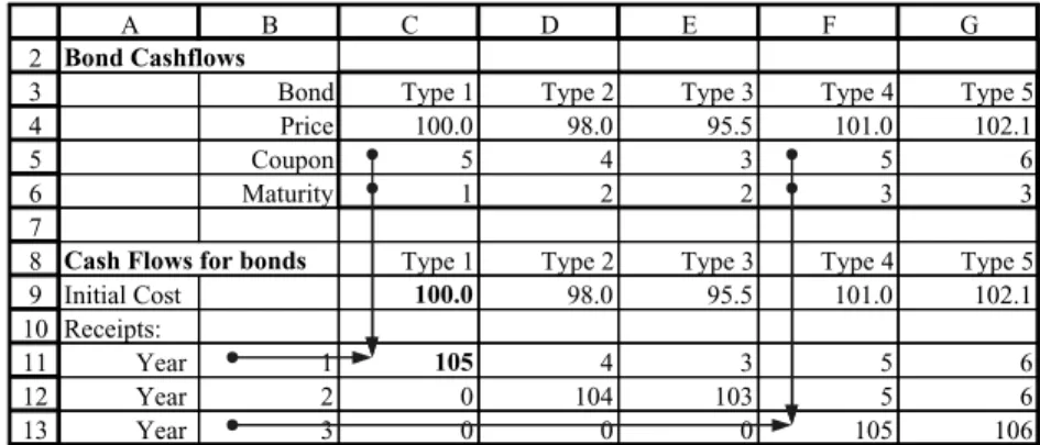
formulas whose syntax takes care of related but different cases. For example, the cash flow in any year for any of the bonds shown in Figure 2.10 could be zero, could be a coupon payment or could be a principal plus coupon payment.
2 3 4 5 6 7 8 9 10 11 12 13 14
A B C D E F G H I
Bond Cashflows
Bond Type 1 Type 2 Type 3 Type 4 Type 5
Price 100.0 98.0 95.5 101.0 102.1
Coupon 5 4 3 5 6
Maturity 1 2 2 3 3
Cash Flows for bonds Type 1 Type 2 Type 3 Type 4 Type 5
Initial Cost 100.0 98.0 95.5 101.0 102.1
Receipts:
Year 1 105 =IF($B11<C$6,C$5,IF($B11=C$6, 100+C$5,0))
Year 2 Year 3
Figure 2.10 A general formula with mixed addressing and nested IF functions in Bonds sheet The IF function gives different outputs for each of two conditions, and a nested IF statement can be constructed to give three outputs (or even more different outputs if
Advanced Excel Functions and Procedures 19 further levels of nesting are constructed). The cash flow formula in cell C11 with one level of nesting:
=IF($B11<C$6,C$5,IF($B11=C$6,100+C$5,0))
produces the cash flows for each bond type and in each year when copied through the range C11:H13.
For the type 1 bond, the cash flow depends on the particular year (cell B11) and the bond maturity (C6). If the year is prior to maturity (B11<C6), the cash flow is a coupon payment C5; if maturity has just been reached (B11DC6), the cash flow is principal plus coupon (100CC5); otherwise (B11>C6), the cash flow is zero. The nested IF takes care of the cash flows when the bond is at (or beyond) maturity, and the first condition in the outer IF takes care of the coupon payments.
The formula is written with ‘mixed addressing’ to ensure that when copied its cell references change appropriately. We write C$6 and C$5 to ensure that when copied down column C, rows 5 and 6 are always referenced for the relevant maturity and premium.
However $B11 will change to $B12 and $B13 for the different years. We write $B11, so that when the formula is copied to column D, column B is still accessed for the year, but C$5 and C$6 change to D$5 and D$6.
The additional thought required to produce this general formula is more than repaid in terms of the time saved when replicating the results for a large model.
2.6 AUDITING TOOLS
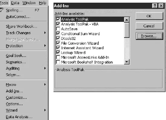
With cell formulas of any complexity, it helps to have the Auditing buttons to hand, i.e.
on a visible toolbar. One way to achieve this from the menubar is via View then Toolbars then Customise. With the Customise dialog box on screen as shown in Figure 2.11, tick the Auditing toolbar, which should then appear.
Figure 2.11 Accessing the Auditing toolbar with main buttons
The crucial buttons are those shown in Figure 2.11, namely from left to right, Trace Precedents, Remove All Arrows and Trace Dependents.
Returning to the spreadsheet, select cell C11 and click the Trace Precedents button to show the cells whose values feed into cell C11 as shown in Figure 2.12. (It also shows the cells feeding into F13.) Click Remove All Arrows to clear the lines.
2 3 4 5 6 7 8 9 10 11 12 13
A B C D E F G
Bond Cashflows
Bond Type 1 Type 2 Type 3 Type 4 Type 5
Price 100.0 98.0 95.5 101.0 102.1
Coupon 5 4 3 5 6
Maturity 1 2 2 3 3
Cash Flows for bonds Type 1 Type 2 Type 3 Type 4 Type 5
Initial Cost 100.0 98.0 95.5 101.0 102.1
Receipts:
Year 1 105 4 3 5 6
Year 2 0 104 103 5 6
Year 3 0 0 0 105 106
Figure 2.12 Illustration of Trace Precedents used on the Bonds sheet
The Customise dialog box is where you can tailor toolbars to your liking. If you click the Commands tab, and choose the appropriate category, you can drag tools from the Commands listbox by selecting and dragging buttons onto your toolbars. Conversely, you can remove buttons from your toolbars by selecting and dragging (effectively returning them to the toolbox).
2.7 DATA TABLES
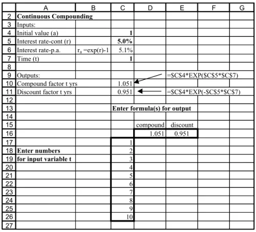
Data Tables help in carrying out a sequence of recalculations of a formula cell without the need to re-enter or copy the formula. The AMFEXCEL workbook contains several examples of Data Tables. We use the calculation of compounding and discounting factors in sheet CompoundDTab to illustrate Data Tables with one input variable, and also with two input variables. A further sheet called BSDTab contains other examples on the use of Data Tables for consolidation.
2.7.1 Setting Up Data Tables with One Input
Figure 2.13 shows the compounding factor for continuous compounding at rate 5% for a period of one year (in cell C10). The equivalent discount factor at rate 5% for one year is in cell D10. The cell formulas for these compounding factors are also shown.
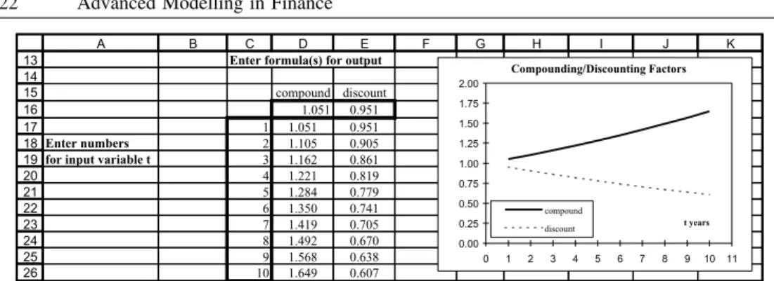
Suppose we want a table of compounding and discounting factors for different time periods, say tD1,2, up to 10 years. To do this via a Data Table, an appropriate layout is first set up, as shown in row 16 and below.
The formula(s) for recalculation are in the top row of the table (row 16). Thus in D16, the cell formula is simply DC10, which links the cell to the underlying formula in
Advanced Excel Functions and Procedures 21 cell C10. Similarly, in E16, the cell formula isDC11. The required list of times for input value t is in column C starting on the row immediately below the formula row. Notice that cell C16 at the intersection of the formula row and the column of values is left blank.
The so-called Table Range for the example in Figure 2.13 is C16:E26.
2
3
4
5
6
7
8
9