Interactions in Marine Stratocumulus Clouds
Thesis by Yi-Chun Chen
In Partial Fulfillment of the Requirements for the degree of
Doctor of Philosophy
CALIFORNIA INSTITUTE OF TECHNOLOGY Pasadena, California
2013
(Defended 30 May, 2013)
2013 Yi-Chun Chen All Rights Reserved
To my parents, Li-Huei Chen and Ya-Ping Chuang.
ACKNOWLEDGEMENTS
First of all, I greatly thank my advisor, Prof. John Seinfeld, for offering me the opportunity to explore the fascinating aerosol-cloud interactions using various tools, from modeling, airborne based field observations, to satellite measurements. I thank him for all the guidance and for being so available for students. In addition, I appreciate his sharp perspectives and superb knowledge of science, as well as his patience when things did not work out as expected. I also thank my committee members, Simona Bordoni, Andy Ingersoll, Tapio Schneider, and Graeme Stephens, for their scientific feedback during these years.
The projects in this dissertation were carried out with tremendous assistance from many colleagues and peers. It is my great pleasure to collaborate with Dr. Graeme Stephens and Dr. Matt Christensen from JPL. I thank them for the time and effort of coming to Caltech for discussions with me on a regular basis. Their suggestions, excellent ideas, and knowledge on satellite data were extremely helpful. The two projects related to satellites could not be accomplished without them.
Special thanks go to Matt Christensen for preparing the satellite data and answering my tons of questions. I must also thank Dr. Lulin Xue from NCAR for the assistance in running the large-eddy simulations and very helpful discussion on the analysis. I also thank him and NCAR for giving me the opportunity to be a visiting graduate student in the NCAR Advance Study Program (ASP).
During the four months visiting NCAR in 2011, I was exposed to various fields of research, and my field of vision became broader. I also thank Dr. Roy Rasmussen, Prof. Armin Sorooshian, Dr.
Hailong Wang, Dr. Frank Li, and Dr. Kentaro Suzuki for all the scientific comments and suggestions. Also, during my first year in Caltech, I worked with Prof. Yuk Yung and Dr. Danie Liang; I appreciate their instruction.
I would like to thank everyone in the Seinfeld research group. I received technical assistance from other modelers, and very much enjoyed the modelers’ coffee time with them, including Wei- Ting Anne Chen, Andi Zuend, Zach Lebo, Joseph Ensberg, and Renee Mcvay. Also, I am grateful for the friendship during the field campaign with Jill Craven, Matt Coggon, and Andrew Metcalf. It was an awesome field campaign and I enjoyed our time doing research as well as having fun together. I thank Kate Schilling and Xuan Zhang for their friendship; it is great to share the research and life experiences with them. In addition, I appreciate the GPS computing staff, Naveed Near- Ansari and John Lilley, as well as secretaries, Elizabeth Miura Boyd and Yvette Grant, for all the trouble shooting and assistance.
The support from my undergraduate study at National Taiwan University meant a lot to me. I thank Prof. I-I Lin, Prof. Ho Lin, Prof. Jen-Ping Chen, and Prof. Chun-Chieh Wu for the caring and encouragement before and during my graduate study at Caltech. I thank my old friends Chia-Jung Pi, Yi-Hsuan Huang, Wei-Ting Fang, Eunice Jiang, and Grace Lee for the mentally support overseas.
Outside the research lab, I thank the members of the Association of Caltech Taiwanese for organizing various events, including softball games, volleyball games, and gatherings on special holidays. These enriched my life in Pasadena. I also appreciate my previous and current roommates Tiffany Wang and Pei Shih for the great company and friendship. They are the best roommates ever. I would like to give thanks to Kevin Yang for being my companion for over four years and I love the awesome dishes he made. His sense of humor makes daily life full of fun. Also, I sincerely appreciate my church friends for the constant support, both physically and spiritually.
Most importantly, I am extremely grateful for the everlasting love and support from my dear families in Taiwan. I thank my parents for all the caring, trust, and encouragement during these six years. I love chatting with my sister about life, work, interesting and sad things, etc. I am really happy that I did not miss her important moments in life – her wedding, as well as the birth of my lovely nephew. Yet I am sorrowful for my dear grandfather’s death. I will remember his warm and gentle smile always. I would also like to give thanks to my brother, grandmother, aunts, uncles, and cousins for all their love.
ABSTRACT
Marine stratocumulus clouds are generally optically thick and shallow, exerting a net cooling influence on climate. Changes in atmospheric aerosol levels alter cloud microphysics (e.g., droplet size) and cloud macrophysics (e.g., liquid water path, cloud thickness), thereby affecting cloud albedo and Earth’s radiative balance. To understand the aerosol-cloud-precipitation interactions and to explore the dynamical effects, three-dimensional large-eddy simulations (LES) with detailed bin-resolved microphysics are performed to explore the diurnal variation of marine stratocumulus clouds under different aerosol levels and environmental conditions. It is shown that the marine stratocumulus cloud albedo is sensitive to aerosol perturbation under clean background conditions, and to environmental conditions such as large-scale divergence rate and free tropospheric humidity.
Based on the in-situ Eastern Pacific Emitted Aerosol Cloud Experiment (E-PEACE) during Jul.
and Aug. 2011, and A-Train satellite observation of 589 individual ship tracks during Jun. 2006- Dec. 2009, an analysis of cloud albedo responses in ship tracks is presented. It is found that the albedo response in ship tracks depends on the mesoscale cloud structure, the free tropospheric humidity, and cloud top height. Under closed cell structure (i.e., cloud cells ringed by a perimeter of clear air), with sufficiently dry air above cloud tops and/or higher cloud top heights, the cloud albedo can become lower in ship tracks. Based on the satellite data, nearly 25% of ship tracks exhibited a decreased albedo. The cloud macrophysical responses are crucial in determining both the strength and the sign of the cloud albedo response to aerosols.
To understand the aerosol indirect effects on global marine warm clouds, multisensory satellite observations, including CloudSat, MODIS, CALIPSO, AMSR-E, ECMWF, CERES, and NCEP, have been applied to study the sensitivity of cloud properties to aerosol levels and to large scale environmental conditions. With an estimate of anthropogenic aerosol fraction, the global aerosol indirect radiative forcing has been assessed.
As the coupling among aerosol, cloud, precipitation, and meteorological conditions in the marine boundary layer is complex, the integration of LES modeling, in-situ aircraft measurements, and global multisensory satellite data analyses improves our understanding of this complex system.
TABLE OF CONTENTS
Acknowledgements ... iv
Abstract ... vi
Table of Contents ... vii
List of Tables ... viii
List of Figures ... ix
Chapter 1: Introduction and Motivation ... 1
Bibliography ... 6
Chapter 2: Large Eddy Simulation on Marine Stratocumulus Clouds ... 8
2.1 Abstract ... 9
2.2 Introduction ... 10
2.3 Cloud Susceptibility to Aerosol Perturbations ... 14
2.4 Model Description ... 18
2.5 Experimental Design ... 19
2.6 Results ... 21
2.7 Conclusions... 34
2.8 Acknowledgements ... 37
2.9 Bibliography ... 38
Chapter 3: Occurrence of Lower Cloud Albedo in Ship Tracks ... 61
3.1 Abstract ... 62
3.2 Introduction ... 62
3.3 Data Description ... 63
3.4 Results ... 68
3.5 Conclusions... 73
3.6 Acknowledgements ... 75
3.7 Bibliography ... 76
Chapter 4: Satellite Estimate of Global Aerosol Indirect Forcing by Marine Warm Clouds ... 93
3.1 Abstract ... 94
3.2 Introduction ... 94
4.3 Data Description ... 96
4.4 Results ... 98
4.5 Aerosol Indirect Radiative Forcing ... 103
4.6 Conclusions... 106
4.7 Bibliography ... 108
LIST OF TABLES
Number Page
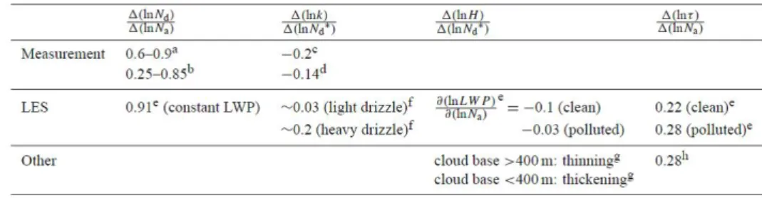
Table 2.1 Studies of aerosol-cloud interactions in MSc. ... 44 Table 2.2 Sign and magnitude of each term in Eq. (2.3) from previous studies ... 44 Table 2.3 Summary of simulated cases ... 45 Table 2.4 Estimation of aerosol-induced effects on MSc cloud properties from the LES model and of cloud susceptibility from Eq. (3) for specific sensitivity simulations under nighttime (4–7 h) and daytime (12–15 h) conditions; aerosol number concentrations considered are 100, 200, 500, and 1000 cm−3.. ... 45 Table 2.5 Values of environmental variables. ... 45 Table 3.1 Instrumentation Payload on CIRPAS Twin Otter. ... 82 Table 3.2 Aerosol/cloud properties measured during E-PEACE Research Flights 18, 19, 20, and 24. For the cloud structure, closed/open means closed or open cloud cellular structure. Cloud layer is defined with cloud droplet number concentration > 10 cm−3 and liquid water content > 0.01 gm−3. Mean Na, Nd, re (cloud drop effective radius), and k (droplet spectral shape parameter) are geometric mean values. BL average w’w’ is the mean vertical velocity variance in the boundary layer. Standard deviation is in parenthesis. ... 83 Table 3.3 Cloud LWP, optical properties, and environmental conditions measured during E-PEACE Research Flights 18, 19, 20, and 24. Standard deviation is in parenthesis. ... 84 Table 4.1 Sensors and corresponding parameters used in the analysis, along
with the spatial resolution. All sensors were matched to the nearest CloudSat footprint ... 111 Table 4.2 Screening procedures and resultant data reductions ... 112 Table 4.3 Slope of linear fit between cloud properties and log10(AI), for
non-precipitating, drizzling, and precipitating clouds ... 112 Table 4.4 The estimated aerosol indirect radiative forcing using Eq. (4.4) and
(4.5) for shortwave (SW) and longwave (LW) component, respectively.
The anthropogenic aerosol fraction (Afrc) is estimated using GEMS
and MODIS. (TOA stands for ‘top of atmosphere’.) ... 112
LIST OF FIGURES
Number Page
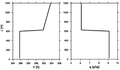
Figure 2.1 Initial sounding profile (potential temperature 𝜃 and total water
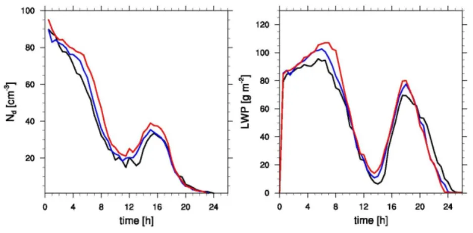
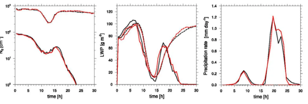
mixing ratio qt ) for the MSc of Control case.. ... 46 Figure 2.2 Time evolution of Nd, LWP, and surface precipitation rate under
different domain size: 2.5×2.5 km2 (black) and 1×1 km2 (red); under
different Na: clean (solid line) and polluted (dashed line) cloud. ... 47 Figure 2.3 Time evolution of Nd and LWP under different vertical spacing:
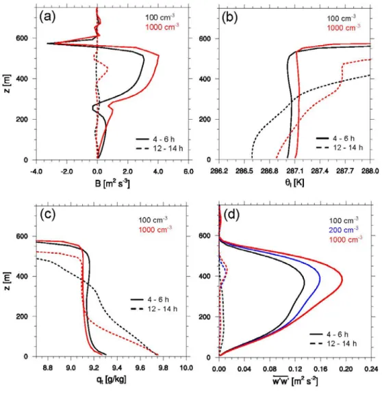
20m (black), 10m (blue), and 5m (red) for clean condition. ... 47 Figure 2.4 Vertical profile averaged over 4–6 h (solid line) and 12–14 h (dashed line) of (a) mean buoyancy flux, 𝐵=𝜃𝑔
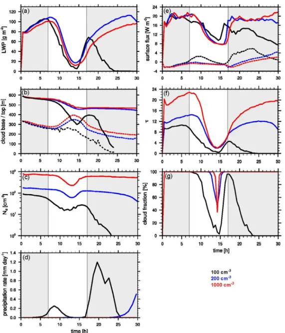
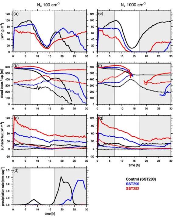
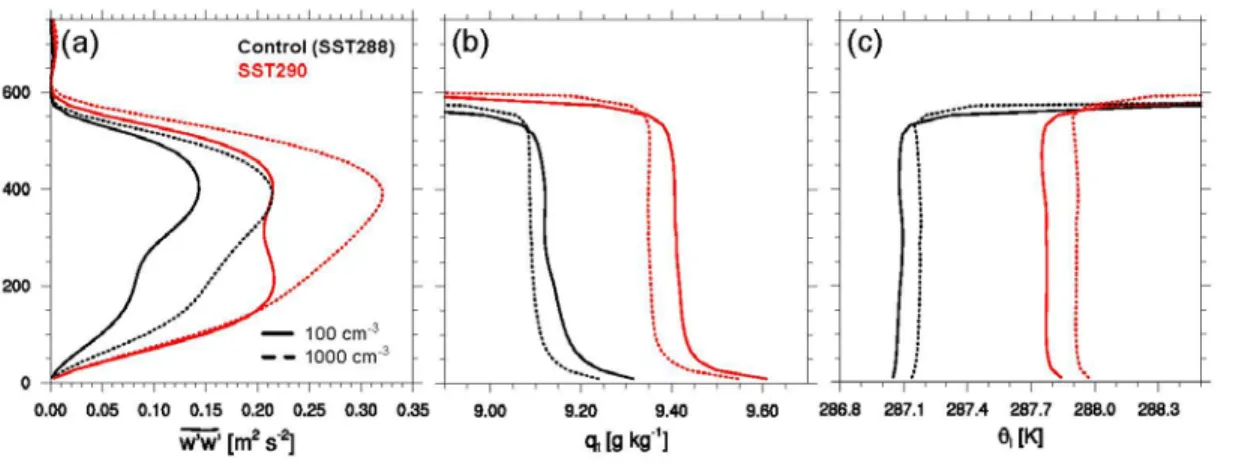
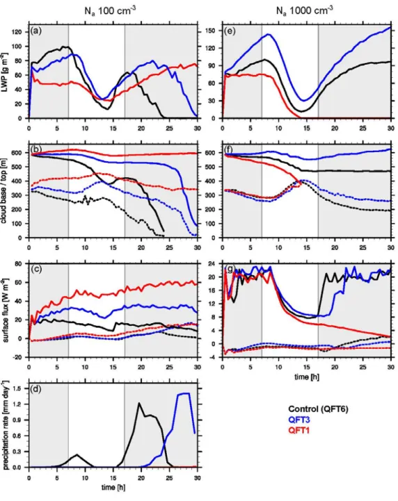
���𝑣𝑤′𝜃�������𝑣′× 10−4, where 𝜃𝑣 is virtual potential temperature, (b) mean liquid water potential temperature 𝜃𝑙 , (c) mean total water mixing ratio qt , and (d) mean vertical velocity variance of clean (black), semi-polluted (blue), and polluted (red) cloud. ... 48 Figure 2.5 Time evolution of clean (Na = 100 cm−3, black), semi-polluted (Na = 200 cm−3, blue), and polluted (Na = 1000 cm−3, red) cloud (2.5×2.5 km2 horizontal domain): (a) average LWP; (b) average cloud top (solid line) and cloud base (dashed line) height, where the cloudy grid is defined as grid with cloud water mixing ratio > 0.01 g kg−1; (c) cloud droplet number concentration Nd, averaged over the cloudy grid; (d) surface precipitation rate, hourly averaged; (e) domain average surface latent (solid line) and sensible (dashed line) heat flux; (f) average cloud optical depth; (g) cloud fraction, defined by cloud optical depth > 2. Gray regions are for the nighttime conditions (0–7 h and 17–30 h), while write regions are for the daytime conditions (7–17 h). ... 49 Figure 2.6 Time evolution of 1×1 km2 clean (Na =100 cm−3, left column) and polluted (Na =1000 cm−3, right column) cloud for Control (black), SST290 (blue) and SST292 (red) case: (a) and (e) average LWP; (b) and (f) average cloud top/base height; (c) and (g) domain average surface latent (solid line) and sensible (dashed line) heat flux; (d) surface precipitation rate, hourly averaged. ... 50 Figure 2.7 Vertical profile averaged over 4–6 h of (a) mean vertical velocity variance, (b) mean total water mixing ratio qt, and (c) mean liquid water potential temperature 𝜃l for Control (black)/SST290 (red) and clean (solid line)/polluted (dashed line) case... 51 Figure 2.8 The same as Fig. 6, except for Control (black), QFT3 (blue) and
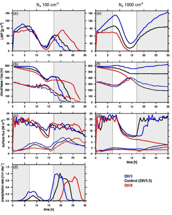
QFT1 (red) case ... 52 Figure 2.9 The same as Fig. 6, except for Control (black), DIV3 (blue) and
DIV8 (red) case... ... 53
Figure 2.10 The same as Fig. 6, except for Control (black) and WIND (red) case.. 54 Figure 2.11 Time evolution of LWP difference between polluted and clean
condition for Control (black), SST290 (red solid), SST292 (red dashed), QFT3 (green solid), QFT1 (green dashed), DIV3 (blue solid), DIV8 (blue dashes), and WIND (orange) case... ... 55 Figure 2.12 Averaged optical depth (τ), cloud droplet number concentration (Nd), dispersion coefficient (k) and cloud thickness (H) as a function of aerosol number concentration Na. Values are averaged horizontally and vertically between cloud top and base for Control (black), SST290 (red), QFT3 (blue), and DIV3 (green) cases during nighttime (averaged over 4–7 h, filled circle) and daytime (average over 12–15 h, cross).... ... 56 Figure 2.13 Averaged Δ(lnτ)/ Δ (lnNa) from the LES model (unfilled circle) and Eq. (2.3) (asterisk) for specific sensitivity simulations under nighttime (4–
7 h) and daytime (12–15 h), as shown in last two columns of Table 2.4.
The error bar (standard deviation) is computed from LES experiments... ... 57 Figure 2.14 The buoyancy integral ratio (BIR) for clean (Na = 100 cm−3) nighttime (4–7 h, black), clean daytime (12–15 h, black open circle), polluted (Na = 1000 cm−3) nighttime (red), and polluted daytime (red open circle) clouds under different environmental conditions. The dashed line corresponds to critical value 0.15 (suggested by Bretherton and Wyant (1997))... ... 58 Figure 2.15 The mean ratio of second to first indirect effect (RIE) for Na from 100 to 200 cm−3 as a function of (a) cloud base height, and (b) cloud thickness.
The data points are averaged over 4–7 h... ... 59 Figure 2.16 The mean ratio of second to first indirect effect (RIE) for Na from 100 to 200 cm−3 during nighttime (4–7 h, black filled circle) and daytime (12–
15 h, circle with cross inside), and from 200 to 1000 cm−3 during nighttime (asterisk) and daytime (triangle)... ... 60 Figure 3.1 Spiral soundings of clean and ship exhaust perturbed areas in E-PEACE research flight 20 and 24 (4 and 10 August 2011, respectively). Flight path is colored according to aerosol number concentration (particle diameter >
120 nm)... ... 85 Figure 3.2 Cloud microphysical parameters measured along the flight tracks. Each symbol represents data over a 1 s increment. Cloud droplet number
concentration [cm−3] is colored on a logarithmic scale; droplet effective radius (re) is given by the size of symbols varying between ~ 4 and 19 μm.
Clean and perturbed cloud data are presented by crosses and open circles, respectively. ... 86 Figure 3.3 GOES satellite images. Satellite images during (a) RF20 (4 August 2011) and (b) RF24 (10 August 2011) off coast of Monterey, CA, exemplifying open and closed cell cloud structures, respectively. Flight path is colored according to aerosol number concentration (particle diameter > 10 nm).. ... 87 Figure 3.4 Magnitude of cloud susceptibility in four E-PEACE cases. Twomey effect (red circle), dispersion effect (green circle), cloud thickness effect (blue circle), and total cloud albedo susceptibility based on Eq. (3.3) (black
circle) and Eq. (3.1) (black cross) for RF18, RF24, RF19, and RF20 (order from low to high cloud albedo susceptibility). ... 88 Figure 3.5 Frequency distribution of different parameters for 589 individual ship tracks from June 2006–December 2009 A-Train observations. The parameters include: (a) dew point depression, (b) cloud top height, (c) effective radius, and (d) optical depth. Albedo enhancement (brightening) and decrease (dimming) cases are shown by red and blue lines, respectively. Means and (standard deviations) are given at the top of each panel. The cloud top height, effective radius, and optical depth are averaged over the unpolluted cloudy sections of each ship track. ... 89 Figure 3.6 Fractional change in cloud albedo (Eq. 3.4) versus the fractional change in logarithm LWP. Indicated are the regime of the Twomey effect (red dots, defined by the absolute value of the fractional change in LWP less than 5 %) and of LWP feedback adjustment (black dots, in which clouds interacted with the environment, resulting in change in LWP). The four E-PEACE data points (pink) are shown.. ... 90
Figure 3.7 Binned change in albedo, effective radius (re), LWP, and cloud thickness (H) as a function of cloud top height (left panel), and dew point depression (right panel) based on 589 ship tracks observed over June 2006-December 2009. Cases were binned by 200 m wide bins in cloud top height and 5 K wide bins in dewpoint depression. A minimum of 20 ship tracks was required for each bin. Error bars were determined from the standard deviation of average cloud albedos taken from the population of ship tracks in each bin. The length of the error bars extends over two standard deviations; i.e., the bar extends one standard deviation below and one above the mean for each bin.. ... 91 Figure 3.8 Conceptual diagram displaying the interactions among aerosol, cloud, precipitation, and meteorology. The response of each property/phenomenon to increased aerosol (Na) is shown as a red plus (signifying positive response), and a blue minus (negative response) sign.
Footnotes to figure: (1) Twomey effect (Twomey, 1991). (2) Albrecht effect (Albrecht, 1989). (3) Sedimentation-entrainment effect (Bretherton et al., 2007).
(4) Drizzle-entrainment effect (Wood, 2007). (5) Significant meteorological conditions, such as free tropospheric humidity (qft), large scale divergence rate, as well as cloud top height (zi), can control the MSc structure (Wood, 2007;
Chen et al., 2011)... ... 92 Figure 4.1 Global relationships between AI and aerosol/cloud parameters for non- precipitating, drizzling, and precipitating clouds. Squares represent the mean values and error bars show the standard deviation.... ... 113 Figure 4.2 Distribution of the least square fitting slope between cloud parameters and log10(AI) with 4°×4° gridded regions. The cloud parameters are: (A) Cloud effective radius, (B) LWP, (C) Cloud thickness, and (D) cloud optical depth. ... 114 Figure 4.3 Distribution of environmental conditions and GEMS anthropogenic aerosol fraction. The environmental variables include: (A) AMSR-E column water vapor, (C) Probability of precipitation, (D) Free tropospheric humidity, (E) Lower tropospheric stability, and (F) 500 mb vertical velocity (represented
as omega). GEMS anthropogenic aerosol fraction is shown in (B).. ... 115 Figure 4.4 Slope of (A) LWP versus log10(AI) and (B) Cloud optical depth (τ) versus log10(AI) under different environmental conditions for non- precipitating clouds. The x-/y-axis correspond to different free
tropospheric relative humidity/lower tropospheric stability, respectively.
Each colored pixel represents the slope that is statistically significant at the 95% confidence interval ... 116 Figure 4.5 Slope of (A) Re versus log10(AI), (B) LWP versus log10(AI), (C) Cloud optical depth versus log10(AI), and (D) Cloud albedo versus log10(AI), under different environmental conditions for precipitating (red) and non- precipitating clouds (black) ... 117 Figure 4.6 Cloud albedo susceptibility (i.e., change in cloud albedo to change in logarithm AI) versus LWP susceptibility. Each data point corresponds to each 4°×4° gridded region ... 118
Chapter 1
Introduction and Motivation
Aerosols influence the microphysical properties of clouds and hence affect their radiative properties, amount and lifetime (IPCC, 2007). This influence, termed the aerosol indirect effect on climate, is identified as one of the major uncertainties in a quantitative assessment of the anthropogenic radiative forcing of climate. Marine stratocumulus clouds (MSc) play a significant role in the Earth’s radiation budget. Covering about one-third of the world’s oceans (Warren et al., 1988), MSc are particularly susceptible to the effect of aerosol perturbations. These clouds are generally optically thick and exist at a low altitude, making them more effective at reflecting solar radiation (albedo is about 30–40%, Randall et al., 1984) than at trapping terrestrial radiation. It has been estimated that a 6% increase of the albedo in MSc regions (equivalent to about a 0.2 g kg-1 moistening of the marine boundary layer (MBL), or an increase in cloud droplet number concentration Nd from 75 to 150 cm-3) could result in a 1 W m-2 change in the net solar radiation at the top of the atmosphere (Stevens and Brenguier, 2009).
The complex interactions of the cloud system involve aerosol and cloud microphysics, atmospheric dynamics, radiation, and chemistry. A number of effects of aerosol perturbations on cloud LWP, cloud lifetime, and precipitation have been predicted by numerical studies and, in some cases, identified by measurements. Overall, the causality that has been proposed for aerosol-cloud-precipitation interactions can be summarized as follows:
(a) Twomey effect (assumes constant LWP): aerosol number concentration (Na) increase smaller, more numerous droplets higher albedo (Twomey, 1977)
(b) Albrecht effect (drizzling cloud): Na increase smaller, more numerous droplets reduced collision-coalescence less precipitation LWP increase higher albedo (Albrecht et al., 1989)
(c) Drizzle-entrainment effect (drizzling cloud): Na increase smaller, more numerous droplets reduced collision-coalescence less precipitation reduced below-cloud evaporative cooling and in-cloud latent heat release higher turbulent kinetic energy (TKE) stronger entrainment LWP decrease lower albedo (e.g., Lu and Seinfeld, 2005; Wood, 2007)
(d) Sedimentation-entrainment effect (non-drizzling cloud): Na increase smaller, more numerous droplets reduced in-cloud sedimentation increase of cloud water and evaporation in entrainment regions stronger entrainment LWP decrease lower albedo (Ackerman et al., 2004; Bretherton et al., 2007; Hill et al., 2009)
(e) Evaporation-entrainment effect (non-drizzling cloud): Na increase smaller, more numerous droplets more efficient evaporation higher TKE stronger entrainment LWP decrease lower albedo (Wang et al., 2003; Xue and Feingold, 2006; Hill et al., 2008)
Drizzle formation leads to release of latent heat in the cloud and to stabilization of the sub- cloud layer through evaporative cooling and moistening. Thus the existence of drizzle reduces the buoyancy, stabilizes the MBL, decreases the TKE, and reduces the entrainment strength. As a result, precipitation suppression due to increased Na increases the buoyancy fluxes and TKE, destabilizes the MBL, and enhances the cloud-top entrainment (as shown in pathway (c)) (e.g., Stevens et al., 1998; Ackerman et al., 2004; Lu and Seinfeld, 2005;
Wood, 2007).
Aerosol-cloud interactions in non-drizzling MSc can be influenced by two kinds of entrainment effects (Hill et al., 2009): (d) Sedimentation-entrainment effect: increasing Na
in nondrizzling MSc reduces in-cloud sedimentation, and thus increases the cloud liquid water content and evaporation in the entrainment region, leading to stronger entrainment and LWP reduction (Bretherton et al., 2007); (e) Evaporation-entrainment effect: increase in Na results in smaller, more numerous cloud droplets, and thus stronger evaporation, which enhances in-cloud turbulence and cloud-top entrainment. The entrained warm, dry air leads to cloud thinning and LWP reduction (Wang et al. 2003; Xue and Feingold 2006).
For both effects an increase in Na leads to LWP reduction, counteracting (b).
The common premise that clouds and precipitation are strongly sensitive to aerosol perturbations neglects the mechanisms that buffer the effects of aerosol perturbations (Stevens and Feingold, 2009). As both aerosol and meteorology (i.e., large-scale dynamic and thermodynamic state) govern the cloudiness, the intertwining of these two factors complicates the interpretation of data (Stevens and Brenguier, 2009).
To represent both MSc microphysics and dynamics, large-eddy simulations (LES) have become a powerful tool because of the ability to realistically represent the larger eddy turbulence field and the interactions of turbulence, cloud microphysics and radiation at an appropriate grid resolution. In order to obtain a comprehensive view of these interactions, high-resolution LES simulations are carried out in Chapter 2 of this thesis. The aerosol- cloud responses under different meteorological factors (include SST, free-tropospheric humidity, large scale subsidence rate, and wind speed) are investigated.
Based on the assumption that increasing aerosol number concentration leads to higher cloud droplet number concentration and an increase in cloud albedo, a marine geo- engineering scheme was proposed (Salter et al., 2008): using wind-driven spray-vessels that pump sub-micrometer sea-salt particles into the air beneath MSc. However, cloud macrophysical responses to increased aerosol levels can lead to either enhancement or diminution of cloud brightening. One of the challenges in understanding the cloud macrophysical responses lies in untangling the aerosol effects from others such as meteorological conditions. In Chapter 3, by utilizing both in situ aircraft measurements E- PEACE (Eastern Pacific Emitted Aerosol Cloud Experiment) and A-Train satellite data, we present an analysis of the factors that control the sign and magnitude of the aerosol indirect effect in ship tracks.
After applying LES study and ship track observations to investigate the aerosol-cloud relationships in regional scale, it is of great interest to understand whether these responses have a global impact. In Chapter 4, to understand the aerosol indirect effects on global marine warm clouds, multisensory satellite observations, including CloudSat, MODIS, CALIPSO, AMSR-E, ECMWF, CERES, and NCEP, have been applied to study the sensitivity of cloud properties to aerosol levels and to large scale environmental conditions. Over the world's oceans for the period August 2006 to December 2009, over 130 million pixels are comprised, of which ~ 3.7 million pixels pass screening for single- layer marine warm clouds. With an estimate of anthropogenic aerosol fraction, the global aerosol indirect radiative forcing has been assessed.
As the coupling among aerosol, cloud, precipitation, and meteorological conditions in the marine boundary layer is complex, the integration of LES modeling, in-situ aircraft
measurements, and global multisensory satellite data analyses improves our understanding of this complex system.
Bibliography
Ackerman, A. S., Kirkpatrick, M. P., Stevens, D. E., and Toon, O. B.: The impact of humidity above stratiform clouds on indirect aerosol climate forcing, Nature, 432, 1014- 1017, 2004.
Albrecht, B.: Aerosols, cloud microphysics, and fractional cloudiness, Science, 245, 1227- 1230, 1989.
Bretherton, C. S., Blossey, P. N., and Uchida, J.: Cloud droplet sedimentation, entrainment efficiency, and subtropical stratocumulus albedo. Geophys. Res. Lett., 34, L03813, doi:10.1029/2006GL027648, 2007.
Hill, A. A., Dobbie, S., and Yin, Y.: The impact of aerosols on non-precipitating marine stratocumulus: Part 1. Model description and prediction of the indirect effect, Q. J. Roy.
Meteor. Soc., 134, 1143-1154, 2008.
Hill, A. A., Feingold, G., and Jiang, H.: The influence of entrainment and mixing assumption on aerosol-cloud interactions in marine stratocumulus, J. Atmos. Sci., 66, 1450- 1464, 2009.
IPCC: Summary for policymakers, in: Climate Change 2007: The Physical Science Basis, Contribution of Working Group I to the Fourth Assessment Report of the Intergovernmental Panel on Climate Change, edited by: Solomon, S., Qin, D., Manning, M., Chen, Z., Marquis, M., Averyt, K. B., Tignor, M., and Miller, H. L., Cambridge University Press, 2007.
Lu, M.-L. and Seinfeld, J. H.: Study of the aerosol indirect effect by Large-Eddy Simulation of marine stratocumulus, J. Atmos. Sci., 62, 3909-3932, 2005.
Randall, D. A.: Stratocumulus cloud deepening through entrainment, Tellus, 36, 446–457, 1984.
Salter, S., Sortino, G., and Latham, J.: Sea-going hardware for the cloud albedo method of reversing global warming, Philos. Trans. Roy. Soc. London, 366, 3989–4006, doi:10.1098/rsta.2008.0136, 2008.
Stevens, B., Cotton, W. R., Feingold, G., and Moeng, C.-H.: Large-eddy simulations of strongly precipitating, shallow, stratocumulus-toped boundary layers, J. Atmos. Sci., 55, 3616-3638, 1998.
Stevens, B. and Brenguier, J.-L.: Cloud controlling factors: low clouds. Clouds in the perturbed climate system, Heintzenberg, J. and Charlson, R. J., The MIT Press, Cambridge, Massachusetts, 173-196, 2009.
Stevens, B. and Feingold, G.: Untangling aerosol effects on clouds and precipitation in a buffered system, Nature, 461, 607-613, 2009.
Twomey, S.: The influence of pollution on the shortwave albedo of clouds, J. Atmos. Sci., 34, 1149-1152, 1977.
Wang, S., Wang, Q., and Feingold, G.: Turbulence, condensation, and liquid water transport in numerically simulated nonprecipitating stratocumulus clouds. J. Atmos. Sci., 60, 262-278, 2003.
Warren, S. G., Hahn, C. J., London, J., Chervin, R. M., and Jenne, R. L.: Global distribution of total cloud cover and cloud type amounts over the ocean. NCAR Tech. Note NCAR/TN-317+STR, 42 pp., 1988.
Wood, R.: Cancellation of aerosol indirect effects in marine stratocumulus through cloud thinning, J. Atmos. Sci., 64, 2657-2669, 2007.
Xue, H., and Feingold, G.: Large-eddy simulations of trade wind cumuli: Investigation of aerosol indirect effects. J. Atmos. Sci., 63, 1605-1622, 2006.
Chapter 2
Large Eddy Simulation
on Marine Stratocumulus Clouds
Published in Atmospheric Chemistry and Physics: Chen, Y.-C., Xue, L., Lebo, Z. J., Wang, H., Rasmussen, R. M., and Seinfeld, J. H.: A comprehensive numerical study of aerosol-cloud-precipitation interactions in marine stratocumulus, Atmos. Chem. Phys., 11, 9749–9769, doi:10.5194/acp-11-9749-2011, 2011.
2.1 Abstract
Three-dimensional large-eddy simulations (LES) with detailed bin-resolved microphysics are performed to explore the diurnal variation of marine stratocumulus (MSc) clouds under clean and polluted conditions. The sensitivity of the aerosol-cloud-precipitation interactions to variation of sea surface temperature, free tropospheric humidity, large scale divergence rate, and wind speed is assessed. The comprehensive set of simulations corroborates previous studies that (1) with moderate/heavy drizzle, an increase in aerosol leads to an increase in cloud thickness; and (2) with non/light drizzle, an increase in aerosol results in a thinner cloud, due to the pronounced effect on entrainment. It is shown that for higher SST, stronger large-scale divergence, drier free troposphere, or lower wind speed, the cloud thins and precipitation decreases. The sign and magnitude of the Twomey effect, droplet dispersion effect, cloud thickness effect, and cloud optical depth susceptibility to aerosol perturbations (i.e., change in cloud optical depth to change in aerosol number concentration) are evaluated by LES experiments and compared with analytical formulations. The Twomey effect emerges as dominant in total cloud optical depth susceptibility to aerosol perturbations. The dispersion effect, that of aerosol perturbations on the cloud droplet size spectrum, is positive (i.e., increase in aerosol leads to spectral narrowing) and accounts for 3% to 10% of the total cloud optical depth susceptibility at nighttime, with greater influence in heavier drizzling clouds. The cloud thickness effect is negative (i.e., increase in aerosol leads to thinner cloud) for non/light drizzling cloud and positive for a moderate/heavy drizzling clouds; the cloud thickness effect contributes 5% to 22% of the nighttime total cloud susceptibility. Overall, the total cloud optical depth susceptibility ranges from ~0.28 to 0.53 at night; an increase in aerosol concentration enhances cloud optical depth, especially with heavier precipitation and in a more pristine environment. During the daytime, the range of magnitude for each effect is more variable owing to cloud thinning and decoupling. The good agreement between LES experiments and analytical formulations suggests that the latter may be useful in evaluations of the total cloud susceptibility. The ratio of the magnitude of the cloud thickness effect to that of the Twomey effect depends on cloud base height and cloud thickness in unperturbed (clean) clouds.
2.2 Introduction
Aerosols influence the microphysical properties of clouds and hence affect their radiative properties, amount and lifetime (IPCC, 2007). This influence, termed the aerosol indirect effect on climate, is identified as one of the major uncertainties in a quantitative assessment of the anthropogenic radiative forcing of climate. Marine stratocumulus clouds (MSc) play a significant role in the Earth’s radiation budget. Covering about one-third of the world’s oceans (Warren et al., 1988), MSc are particularly susceptible to the effect of aerosol perturbations. These clouds are generally optically thick and exist at a low altitude, making them more effective at reflecting solar radiation (albedo is about 30–40%, Randall et al., 1984) than at trapping terrestrial radiation. It has been estimated that a 6% increase of the albedo in MSc regions (equivalent to about a 0.2 g kg-1 moistening of the marine boundary layer (MBL), or an increase in cloud droplet number concentration Nd from 75 to 150 cm-3) could result in a 1 W m-2 change in the net solar radiation at the top of the atmosphere (Stevens and Brenguier, 2009).
The complex interactions of the cloud system involve aerosol and cloud microphysics, atmospheric dynamics, radiation, and chemistry. The dynamics of MSc have been the subject of numerous modeling studies. Mixed-layer models (MLMs, Lilly, 1968) couple cloud, radiation, and turbulence to describe the cloud-topped marine boundary layer (MBL) (e.g., Turton and Nicholls, 1987; Bretherton and Wyant, 1997; Lilly, 2002; Wood, 2007;
Sandu et al., 2009; Caldwell and Bretherton, 2009a; Uchida et al., 2010). Given surface and free-tropospheric thermodynamic conditions, bulk cloud properties, such as thickness, cloud liquid water path (LWP), and the MBL steady-state, can be determined by an MLM.
The MLM framework represents a well-mixed MBL. Departures from well-mixed conditions are, however, common in situations of precipitation and during daytime.
To represent both MSc microphysics and dynamics, large-eddy simulations (LES) have become a powerful tool because of the ability to realistically represent the larger eddy turbulence field and the interactions of turbulence, cloud microphysics and radiation at an appropriate grid resolution. LES has been applied in many previous studies of MSc (e.g., Stevens et al., 1998; 2003; 2005; Stevens and Bretherton, 1999; Bretherton et al., 1999;
Chlond and Wolkau, 2000; Jiang et al., 2002; Wang et al., 2003; Duynkerke et al., 2004; Lu
and Seinfeld, 2005, 2006; Bretherton et al., 2007; Sandu et al., 2008; Savic-jovcic and Stevens, 2008; Yamaguchi and Randall, 2008; Hill et al., 2008; 2009; Ackerman et al., 2009; Caldwell and Bretherton, 2009b; Wang and Feingold, 2009a,b; Wang et al., 2010;
Uchida et al., 2010). Table 2.1 summarizes a number of studies that focus mainly on aerosol-cloud interactions in MSc; these address the LWP responses to changes in aerosol number and ambient environmental conditions, including sea surface temperature (SST), large scale divergence rate (D), and free tropospheric humidity (qft). Atmospheric aerosols and meteorology each exert controls on cloudiness; the former governs the cloud micro- structure, while the latter provides the dynamic and thermodynamic state that controls cloud macro-structure (Stevens and Brenguier, 2009).
A number of effects of aerosol perturbations on cloud LWP, cloud lifetime, and precipitation have been predicted by numerical studies and, in some cases, identified by measurements. Overall, the causality that has been proposed for aerosol-cloud-precipitation interactions can be summarized as follows:
(a) Twomey effect (assumes constant LWP): aerosol number concentration (Na) increase smaller, more numerous droplets higher albedo (Twomey, 1977)
(b) Albrecht effect (drizzling cloud): Na increase smaller, more numerous droplets reduced collision-coalescence less precipitation LWP increase à higher albedo (Albrecht et al., 1989)
(c) Drizzle-entrainment effect (drizzling cloud): Na increase smaller, more numerous droplets reduced collision-coalescence less precipitation reduced below-cloud evaporative cooling and in-cloud latent heat release higher turbulent kinetic energy (TKE) stronger entrainment LWP decrease lower albedo (e.g., Lu and Seinfeld, 2005; Wood, 2007)
(d) Sedimentation-entrainment effect (non-drizzling cloud): Na increase smaller, more numerous droplets reduced in-cloud sedimentation increase of cloud water and evaporation in entrainment regions stronger entrainment LWP decrease lower albedo (Ackerman et al., 2004; Bretherton et al., 2007; Hill et al., 2009)
(e) Evaporation-entrainment effect (non-drizzling cloud): Na increase smaller, more numerous droplets more efficient evaporation higher TKE stronger entrainment LWP decrease lower albedo (Wang et al., 2003; Xue and Feingold, 2006; Hill et al., 2008)
Drizzle formation leads to release of latent heat in the cloud and to stabilization of the sub-cloud layer through evaporative cooling and moistening. Thus the existence of drizzle reduces the buoyancy, stabilizes the MBL, decreases the TKE, and reduces the entrainment strength. As a result, precipitation suppression due to increased Na increases the buoyancy fluxes and TKE, destabilizes the MBL, and enhances the cloud-top entrainment (as shown in pathway (c)) (e.g., Stevens et al., 1998; Ackerman et al., 2004; Lu and Seinfeld, 2005;
Wood, 2007).
Aerosol-cloud interactions in non-drizzling MSc can be influenced by two kinds of entrainment effects (Hill et al., 2009): (d) Sedimentation-entrainment effect: increasing Na
in nondrizzling MSc reduces in-cloud sedimentation, and thus increases the cloud liquid water content and evaporation in the entrainment region, leading to stronger entrainment and LWP reduction (Bretherton et al., 2007); (e) Evaporation-entrainment effect: increase in Na results in smaller, more numerous cloud droplets, and thus stronger evaporation, which enhances in-cloud turbulence and cloud-top entrainment. The entrained warm, dry air leads to cloud thinning and LWP reduction (Wang et al. 2003; Xue and Feingold 2006).
For both effects an increase in Na leads to LWP reduction, counteracting (b).
In simulations of MSc, Ackerman et al. (2004) showed that for moderate/heavy surface precipitation rates the LWP increases with Nd (following effect (b)). On the other hand, under non/light drizzling conditions the LWP decreases with increasing Nd (as explained by pathways (d) and (e)). Similar trends have also been found in other nocturnal studies (Table 2.1), in which opposite responses of LWP to an increase in Na for heavy/moderate and light/non- drizzling conditions occur. The free troposphere moisture (qft) exerts a strong control on the precipitation rate through cloud-top entrainment, thus altering the balance between the competing effects of precipitation on LWP. The effects of the free tropospheric moisture can be summarized (Ackerman et al., 2004) as: (i) moist entrained air does not
dry MBL effectively cloud thickening, versus (ii) dry entrained air dry the MBL cloud thinning. Similar results were also obtained by Sandu et al. (2008) for a diurnal cycle.
The effect of changes in the large scale divergence, D, is consistent among the studies listed in Table 2.1, showing that under higher (lower) D, the cloud top is driven down (higher), resulting in thinner (thicker) cloud, lower (higher) LWP. Since D is difficult to measure, its value is usually estimated.
The effect of changes in SST on MSc has been addressed in several studies. Lu and Seinfeld (2005) and Wood (2007) found that with higher SST, the MBL deepens and cloud base rises, resulting in a thinner cloud with lower LWP. In the LES study of Lu and Seinfeld (2005), the initial temperature in the entire MBL was assumed to increase systematically with SST, and the MBL relative humidity was adjusted as well; the MSc becomes less cloudy because of gradual dissipation. In the MLM study of Caldwell and Bretherton (2009a), however, as SST increases, the equilibrium cloud base and cloud top heights both increase due to increased entrainment through a weaker inversion, resulting in a thicker cloud with higher LWP. Therefore in response to a higher SST, shorter time scale and equilibrium responses have different effects on MSc.
Diurnal variation is the result of competition between cloud top longwave (LW) radiative cooling occurring both day and night, and daytime solar heating (Hill et al., 2008). During nighttime, cloud top LW cooling enhances TKE, couples the cloud and the surface fluxes, well mix the MBL, and the cloud tends to become thicker. While under daytime conditions, absorption of solar radiation offsets the cloud top LW cooling, stabilizing the MBL, causing the cloud to thin; some clouds may even become decoupled. Predicted daytime LWP is consistently smaller than that in nighttime (Table 2.1). Also, daytime MBL is less sensitive to changing Na than under nighttime conditions (e.g., Ackerman et al., 2004; Lu and Seinfeld, 2005), suggesting cloud-radiation interactions are important in controlling the diurnal variation.
From a summary of the studies cited in Table 2.1, overall, non/light drizzling MSc and moderate/heavy drizzling MSc respond differently to changes in aerosol level since the dominant physical/dynamical mechanisms differ. Also, distinct diurnal responses are
shown in day and nighttime conditions as a result of cloud-radiation interactions. And MSc is found to be sensitive to changes in ambient conditions, e.g., SST, D, or qft.
Aerosol-cloud-precipitation interactions in MSc are tightly intertwined and often subtle. In order to obtain a comprehensive view of these interactions, high-resolution LES simulations are carried out in the present study. The meteorological factors investigated include SST, free-tropospheric humidity, large scale subsidence rate, and wind speed.
Diurnal variation is considered as well as non/light drizzling and moderate/heavy drizzling MSc. We begin with an analytical formulation of cloud susceptibility to aerosol perturbation in terms of the Twomey, cloud droplet dispersion, cloud thickness, and diabaticity effects. The sign and magnitude of each effect are evaluated from LES simulations to compare with the analytical formulations. While each of the studies cited in Table 2.1 addresses one or more aspects of aerosol-MSc interactions, the present study is intended to be a comprehensive, consistent evaluation of these interactions covering the range of the important variables.
2.3 Cloud Susceptibility to Aerosol Perturbations
Before proceeding to the numerical study, it is useful to address MSc aerosol-cloud relationship from a simplified analytical point of view, providing a consistent basis on which to connect aerosol-cloud-precipitation interactions. Considering the change of cloud radiative properties in response to a change in aerosol number concentration, Na, the relationship between adiabatic cloud optical thickness τad and adiabatic cloud droplet number concentration, Nad , can be expressed (Brenguier et al., 2000):
𝜏𝑎𝑑 = 9 10 (
4
3𝜋)1/3 𝑙02/3(𝑘 𝑁𝑎𝑑)1/3 𝐻5/3 (2.1) where 𝑙0=𝜌𝐶𝑤
𝑤 , 𝜌𝑤 is the density of water, 𝐶𝑤 is the moist adiabatic condensation coefficient, 𝑘 is a parameter related to the droplet spectrum shape, which is inversely proportional to the droplet distribution breadth, and 𝐻 is cloud thickness. The range of 𝑘 is 1 in the limit of a monodisperse size distribution and approaches 0 for a very wide distribution. In the presence of cloud top entrainment and water loss through precipitation, the cloud droplet profile tends to be diabatic. A sub-adiabaticity parameter 𝑓 can be defined
to include the effects of entrainment and precipitation in drying out the cloud relative to the adiabatic case. Equation (2.1) can be generalized (W. Conant, personal communication) as
𝜏= 9 10 (
4
3𝜋)1/3 𝑙02/3𝑓(2+𝑚)/3(𝑘 𝑁𝑎𝑑)1/3 𝐻5/3 (2.2) where 𝑓 is 1 under adiabatic conditions, and approaches 0 as the degree to which the profile is sub-adiabatic increases. The parameter 𝑚 describes the microphysical impacts of mixing between the cloudy air and the relatively dry/warm free tropospheric air. 𝑚 = 1 corresponds to the limit of inhomogeneous mixing, in which the turbulent mixing is relatively slow and all droplets in the entrained air evaporate, resulting in reduction of Nd
and broadening of the droplet spectrum. 𝑚 = 0 corresponds to the limit of homogeneous mixing, in which the timescale of turbulent mixing is much shorter than that at which droplets respond to the fresh ambient air. In this limit, all droplets experience the same degree of sub-saturation and evaporate together; thus 𝑁𝑑 remains constant as all droplets shift to smaller sizes.
From equation (2.2), the impact of changes in aerosol number concentration on cloud optical depth (the cloud susceptibility) can be expressed as follows:
𝑑𝑙𝑛𝜏 𝑑𝑙𝑛𝑁𝑎=1
3�𝑑𝑙𝑛𝑁𝑎𝑑
𝑑𝑙𝑛𝑁𝑎 + 𝑑𝑙𝑛𝑘
𝑑𝑙𝑛𝑁𝑎+ 5 𝑑𝑙𝑛𝐻
𝑑𝑙𝑛𝑁𝑎+ (2 +𝑚) 𝑑𝑙𝑛𝑓
𝑑𝑙𝑛𝑁𝑎 � (2.3)
2.3.1 Twomey effect
From the above equation, 𝑑𝑙𝑛𝑁𝑎𝑑/𝑑𝑙𝑛𝑁𝑎 represents the so-called Twomey effect. An analytical relationship between 𝑁𝑎𝑑 and 𝑁𝑎, modified from that derived by Twomey (1959), is
𝑁𝑎𝑑 =𝑁𝑎𝑘𝑠2+2[ 𝑐𝑤32 𝑘𝑠𝐵 �𝑘2 ,𝑠 3
2� ]𝑘𝑘𝑠+2𝑠 (2.4) where 𝐵 is the beta function, 𝑤 is updraft velocity at cloud base, 𝑘𝑠 is a parameter related to the exponent in an assumed power-law aerosol size distribution, and 𝑐 is a composition-
dependent parameter that relates the aerosol size distribution to the supersaturation spectrum. From equation (2.4),
𝑑𝑙𝑛𝑁𝑎𝑑 𝑑𝑙𝑛𝑁𝑎 = 2
𝑘𝑠+ 2 (5) Values of 𝑘𝑠 range from 0.3 to 1.4 (empirical constants for cloud condensation nuclei, CCN, at 1 % supersaturation, from Pruppacher and Klett (1997)). For that range, 𝑑𝑙𝑛𝑁𝑎𝑑/ 𝑑𝑙𝑛𝑁𝑎 varies from about 0.6~0.9 under adiabatic conditions. Shao and Liu (2009) compared 𝑑𝑙𝑛𝑁𝑎𝑑/𝑑𝑙𝑛𝑁𝑎 predicted by equation (2.5) with in-situ measurements (values of 0.25~0.85). Differences in the value of 𝑑𝑙𝑛𝑁𝑎𝑑/𝑑𝑙𝑛𝑁𝑎 between the analytical expression and ambient measurements can be attributed to (i) activation effect: adding aerosols, for example, into a marine aerosol background reduces the ability of aerosols to act as CCN, and (ii) adiabaticity influence: the variability of the adiabaticity (cloud dilution state) from different meteorological conditions between clean and polluted clouds.
2.3.2 Dispersion effect
The second term 𝑑𝑙𝑛𝑘/𝑑𝑙𝑛𝑁𝑎expresses the effect of changes in 𝑁𝑎 on the cloud droplet size distribution. Dispersion in the droplet distribution is related to aerosol composition (e.g., Feingold and Chuang, 2002), microphysics (e.g., collision-coalescence), and dynamics (e.g., entrainment mixing, updraft velocity) (Wood et al., 2002; Lu and Seinfeld, 2006). It is noted from observational data (Martin et al., 1994; Ackerman et al., 2000; Liu and Daum, 2002) that the dispersion forcing would lead to an indirect warming effect, opposing the Twomey effect. Accounting for the parameterization of dispersion effect in GCMs leads to a reduction in the magnitude of the predicted Twomey effect (Rotstayn and Liu, 2003, 2009). By contrast, an opposite trend is found in the LES study of Lu and Seinfeld (2006). For a drizzling cloud, increasing Na leads to spectrum narrowing (larger 𝑘) because smaller droplets suppress precipitation formation by limiting the collision- coalescence process and enhance droplet condensational growth in the presence of higher updraft velocities, due to stronger TKE (Lu and Seinfeld, 2006). In that case, the dispersion effect enhances the Twomey effect. This trend is evident in in-situ measurements by Miles et al. (2000) and individual ship tracks in Lu et al. (2007).
2.3.3 Cloud thickness effect
The third term in equation (2.3), 𝑑𝑙𝑛𝐻/𝑑𝑙𝑛𝑁𝑎, expresses the sensitivity of cloud thickness to changes in 𝑁𝑎, for which Wood (2007) derived an analytical formulation and applied a MLM to quantify the response of cloud thickness to perturbed Nd under different environmental conditions. Wood (2007) showed that the MSc cloud thickness response is determined by a balance between the moistening/cooling of the MBL resulting from precipitation suppression and drying/warming resulting from enhanced entrainment due to increased TKE. The drying and warming effect (cloud thinning) counteracts the moistening/cooling effect (cloud thickening). Also using the MLM model, Pincus and Baker (1994) predicted that cloud thickness (𝐻) increases with Nd, especially at lower droplet concentration. Unlike the Pincus and Baker (1994) result that 𝐻 is determined primarily by cloud top height, Wood (2007) found the cloud base height to be the single most important determinant in affecting cloud thickness. If the cloud base height is lower (higher) than 400 m, increasing Nd leads to cloud thickening (thinning), which corresponds to LWP increase (decrease). The argument is that for an elevated cloud base, more evaporation occurs before precipitation reaches the surface, leading to two effects (Wood, 2007): (i) more sub-cloud evaporation limits the moistening/cooling of the MBL resulting from precipitation suppression, while allowing suppressed precipitation to increase the entrainment with increasing Nd, and (ii) sub-cloud evaporation has a stronger effect on turbulence than in-cloud latent heating; therefore enhanced sub-cloud evaporation increases the leverage of changes in cloud base precipitation on entrainment.
2.3.4 Adiabaticity effect
The term, 𝑑𝑙𝑛𝑓/𝑑𝑙𝑛𝑁𝑎, can be termed the diabaticity effect, accounting for the effect of liquid water depletion due to entrainment mixing and precipitation on cloud optical depth.
This term cannot be evaluated separately from the other terms; the effect of diabaticity is intertwined with all the previous effects discussed. The qualitative effect of entrainment mixing on cloud behavior has been discussed in Section 1 (effects (c), (d), and (e)).
Some of these individual effects have been estimated in several previous studies (Table 2.2), including analytical solutions, in-situ measurements, satellite data, and LES. We will subsequently estimate the magnitudes for each effect from LES simulation.
2.4 Model Description 2.4.1 Numerical model
In this study we employ the Weather Research and Forecasting (WRF) model V3.1.1 as a 3D LES model. A detailed bin-resolved microphysical scheme (Geresdi, 1998; Rasmussen et al., 2002; Xue et al., 2010) is employed. In the bin microphysical scheme, aerosol number, cloud drop mass, and cloud drop number are computed over a size-resolved spectrum, predicting both cloud drop mass and number concentration following the moment-conserving technique (Tzivion et al., 1987, 1989; Reisin et al., 1996). Cloud drops are divided into 36 size bins with radii ranging from 1.56 μm to 6.4 mm and with mass doubling between bin. The masses for the first bin and the 36th bin are 1.5979×10⁻¹⁴ and 1.098×10⁻³ kg, respectively. In this study, the cutoff radius between cloud drop and rain drop size is taken to be 40 μm. The aerosols are divided into 40 size bins between 0.006 to 66.2 μm.
2.4.2 Microphysical processes
The microphysical processes include aerosol activation, drop condensation/evaporation, collision-coalescence, collisional breakup, and sedimentation. The aerosol size distribution is taken to be a single mode lognormal size distribution. Aerosol activation (or cloud droplet activation) occurs when the ambient supersaturation exceeds the critical supersaturation (𝑆𝑐) for the given particle size. A hygroscopicity parameter к, which describes the relationship between dry particle diameter and cloud condensation nuclei activity, is used to represent the composition-dependence of the solution water activity (Petters and Kreidenweis, 2006),
𝑆𝑐(𝐷) = 𝐷3− 𝐷𝑑3
𝐷3− 𝐷𝑑3(1− 𝜅)exp�4𝜎𝑠
𝑎𝑀𝑤
𝑅𝑇𝜌𝑤𝐷� −1 (2.6)
where 𝐷 is droplet diameter, 𝐷𝑑 is aerosol dry diameter, 𝜎 is the surface tension of the solution/air interface, 𝑀𝑤 is the molecular weight of water, and 𝜌𝑤 is the density of water.
For the present study, the aerosol is assumed to be ammonium sulfate, for which к is set to the constant value 0.615 (Petters and Kreidenweis, 2006).
The aerosol number concentration is held constant in the present study. Thus we neglect below-cloud precipitation scavenging of aerosol. The activated droplet number at each time is calculated by the difference between the particle number that would be activated at the diagnosed supersaturation and the pre-existing droplet number. Diffusional growth and evaporation of water drops are described following the vapor diffusion equation (Pruppacher and Klett, 1997). The Best and Bond number approach is used to calculate the terminal velocity of water drops (Pruppacher and Klett, 1997). The efficiencies of collision- coalescence between drops are derived using the data of Hall (1980) to calculate the kernel function. The collisional breakup of water drops is included following Feingold et al.
(1988).
2.4.3 Other processes
Surface latent and sensible heat fluxes are calculated from local wind speed and the difference in specific humidity/temperature between the ocean and the air just above the ocean surface, following the Monin-Obukhov scheme. A 3D turbulence scheme with 1.5- order turbulent kinetic energy (TKE) closure (Deardorff, 1980) is applied to prognose TKE.
The Rapid Radiative Transfer Model (RRTM; Mlawer et al., 1997) with 16 LW band is utilized to calculate LW radiative fluxes. The correlated-k method is used to simulate the cloud top radiative cooling and heating rates. Shortwave radiation is represented using the Dudhia scheme (1989) to include solar flux, shortwave absorption and scattering in clear air, and reflection and absorption in cloud layers. A damping layer of 300m thickness is employed in the upper boundary of domain for absorbing gravity wave energy to minimize the unphysical wave reflection off the upper boundary of the domain. Periodic boundary conditions in both x- and y- directions are assumed in the simulations. The monotonic flux limiter is applied to the basic advection scheme for scalar transport, as suggested by Wang et al. (2009) to avoid overestimates of cloud water and precipitation in cloud-scale simulations.
2.5 Experimental Design
The WRF model with detailed bin microphysics is used to simulate an idealized MSc case through a 30 hr diurnal cycle. The aerosol is assumed to be fully soluble ammonium sulfate with lognormal distribution mean radius 0.1 μm and geometric standard deviation 1.5. The
initial sounding profile for the control case (Fig. 2.1) is loosely based on the First International Satellite Cloud Climatology Project Regional Experiment (FIRE I; Duynkerke et al., 2004) in July 1987, with the total water mixing ratio decreased by 0.5 g kg-1 for a moderately drizzling (0.1–1 mm day-1) cloud. The case simulated is a shallow boundary layer with a depth of ~600 m and topped with a 12 K and -3 g kg-1 temperature and moisture inversion, respectively. The Coriolis parameter is 8×10⁻⁵ s-1 (33.5 N, 119.5 W).
Other initial conditions are similar to those in Hill et al. (2009). The nominal sea surface temperature (SST) is set to 288 K, and surface pressure is assumed to be constant at 1012.5 mb. The wind field is -1 m s-1 in the x-direction and 6 m s-1 in the y-direction. The nominal large-scale divergence rate (D), 5.5×10⁻⁶ s-1, is given to prescribe the subsidence rate Wsub=- Dz, where z is the height above surface. The initial temperature field is perturbed pseudo- randomly by an amplitude of 0.1 K to accelerate the spinup of convection. Results are not sensitive to this amplitude. Both LW and SW radiation are considered. Radiative forcing is computed every time step. In order to avoid MSc dissipation due to strong solar radiation in summer, winter conditions are chosen for SW radiation.
The simulations are performed within a 3 km × 3 km × 1.6 km domain for 30 hr. The grid resolution is 20 m vertically and 50 m horizontally, with a 0.5 s time stop. Aerosol number concentrations (Na) of 100, 200, and 1000 cm-3 are taken to correspond to clean, semi- polluted, and polluted cases, respectively. For computational efficiency, sensitivity studies are performed over a smaller horizontal domain size, 1 km in x- and y- directions. Fig. 2.2 shows that the cloud bulk properties of larger (3 km × 3 km) and smaller (1 km × 1 km) domain sizes are similar. Since our focus is on the directional changes of cloud properties in response to different ambient conditions, the smaller domain is sufficient for sensitivity studies. Four significant environmental variables that control the structure of the MSc are considered: SST, free tropospheric water vapor mixing ratio (qft), large-scale divergence rate (D), and wind speed (U and V). The lower BL stability is controlled mainly by SST (Klein and Hartmann, 1993). The humidity above the BL determines the drying/warming effect through entrainment. The large-scale divergence D affects the subsidence rate. The wind speed is considered, as it affects the surface fluxes and the updraft velocity.
The simulations performed are listed in Table 2.3. In cases SST290 and SST292, SST is increased by 2K and 4K, respectively. In cases QFT3 and QFT1, the free tropospheric
water vapor mixing ratio is decreased to 3.1 and 1.1 g/kg, respectively; the temperature profile remains unchanged. In cases DIV3 and DIV8, the large scale divergence rate is set to 3.0×10⁻⁶ and 8.0×10⁻⁶ s-1, respectively, with all else unchanged. In WIND case, the wind speed is set to -4 m/s in the x-direction and 10 in the y-direction, stronger than the Control case. Both clean and polluted scenarios are simulated for each condition.
2.6 Results 2.6.1 Control case
The simulations start at 00:00 h local time. During nighttime, cloud top LW radiative cooling generates positive buoyancy in the cloud layer (Fig. 2.4a), which enhances TKE and mixing, destabilizing the MBL and increasing the cloud top entrainment. Cloud-top entrainment tends to raise the cloud base by diluting the cloud with warm and dry air, but it also tends to lift cloud top height (e.g., Randall, 1984). With stronger mixing, water vapor from the surface is transported to upper layers more efficiently, causing the difference between water vapor mixing ratio at the reference level and saturation mixing ratio at the surface to increase, and thus leading to a higher surface moisture flux. This results in a moister cloud layer, increased cloud thickness and LWP at nighttime (Fig. 2.5a, 2.5b). For the clean case (Na = 100 cm−3), measurable surface precipitation begins at 5 h as LWP increases, proceeding from light drizzle (surface rain rate < 0.1 mm day−1) to moderate drizzle (0.1–1 mm day−1) after 7 h. During the daytime, the heating due to cloud absorption of solar radiation partially offsets the cloud top LW cooling, stabilizing the MBL. Heating of the cloudy layer via SW absorption acts to thin the cloud; surface precipitation is suppressed after 12 h (Fig. 2.5d). Also, the MSc becomes decoupled from the sub-cloud layer as the cloud gets slightly warmer than the sub-cloud layer and a stable layer occurs at the cloud base. In the 𝜃l and qt daytime profiles (Fig. 2.4b, 2.4c), it is shown that the moister and cooler surface air is not transported to the cloud layer effectively (12–14 h). As the cloud continues to warm, the LWP decreases, attaining a minimum at ~14 h. It is noted, however, that the solar heating is likely overestimated with the Dudhia SW radiation scheme and leads to overly reduced daytime cloud water.
After 14 h, cloud top height begins to increase again due to a decrease in downwelling SW radiation, and drizzle appears after ~16 h (Fig. 2.5d). In the clean case, the drizzle
evaporation below the cloud can moisten and cool the sub-cloud layer, increasing the relative humidity of the sub-cloud air, lowering the cloud lifting condensation level, hence lowering cloud base (Lu and Seinfeld, 2005). Also, the cloud-top entrainment decreases in the presence of drizzle, therefore the cloud top falls. The decreased entrainment drying/
warming increases the MBL relative humidity and leads to a lower lifting condensation level. Therefore, more raindrops are likely to reach the surface before evaporating in the sub-cloud layer. As the surface precipitation increases during the second night, the cloud becomes optically thinner (Fig. 2.5f) and cloud top LW cooling decreases, allowing subsidence to compress the MBL. The cloud eventually disappears at ~24 h.
Proceeding from clean to semi-polluted (Na =200 cm−3) condition, more numerous and smaller cloud droplets undergo less efficient collision-coalescence, which leads to a suppression of precipitation. Therefore, the semi-polluted case is nonprecipitating for the first 25 h. The precipitation suppression at nighttime results in higher TKE, because in the presence of precipitation, drizzle formation leads to stabilization of the sub-cloud layer through evaporative cooling and moistening. The cooling and moistening below the cloud leads to weaker turbulence intensity and inhibition of deeper mixing, and may also lower the cloud base (Lu and Seinfeld, 2005). During the daytime this can partially offset the warming of the cloud base due to absorption of solar radiation and counteract the tendency for the cloud base to rise (Sandu et al., 2008). The existence of drizzle reduces the buoyancy, stabilizes the MBL, decreases the TKE, and reduces the entrainment strength.
As a result, precipitation suppression due to increased Na increases the buoyancy fluxes and TKE, destabilizes the MBL, enhances the cloud-top entrainment (as shown in pathway (c)), and establishing a well-mixed MBL. This is consistent with previous findings (e.g., Stevens et al., 1998; Ackerman et al., 2004; Lu and Seinfeld, 2005; Wood, 2007).
From 10 to 15 h, the semi-polluted cloud thins due to solar heating. With a stabilized MBL and decreased TKE during the daytime, the cloud top falls by 80m due to reduced cloud top entrainment. As the MBL gradually warms with SW heating, the relative humidity in the MBL decreases, causing the cloud base to rise by 100 m. Consequently, LWP decreases as cloud thins. During the second night, the LWP of the semi-polluted cloud increases with weaker SW heating, exceeding 110 g m−2, and drizzle appears in the last 5 h of the simulation.