Analysis of Packaging and Deployment of Ultralight Space Structures

Also shown is a close-up of the area where the ribbon spring buckled when in contact with four-sided shell elements. 88 5.5 (a) Schematic representation of experimental setup for measuring the coefficient of friction between. the hub and the ribbon spring.

Overview

Deployable Structures

Testing of Deployable Structures

However, there is still air resistance, which can be problematic for laying out thin-film structures, such as solar sails. Once the model is validated, gravity and drag can be removed from the model and the performance in space estimated.

Analytical and Numerical Models of Deployable Structures

Halfway between ground testing and space testing lie drop towers and gravity flights. The effects of atmospheric drag can be reduced by pumping out the air, although there will always be some residual drag [22].

Objective and Scope

Layout of Dissertation

Large Planar Thin-Film Structures

Since the force transmitted by light is extremely small, solar sails must be very large and light. Because these arms also need to be packed into a tight configuration, all of these arms themselves are also ultralight adjustable space structures.

Strain Energy Deployed Booms

The UN guidelines for space debris reduction state that satellites must be de-orbited within 25 years of their intended lifetime [15] or moved to a graveyard orbit above 2000 km. When equipped with a drag sail, the projected area of the satellite increases significantly, increasing atmospheric drag and leading to a much faster de-orbit.

Coilable Deployable Booms

Additional modifications are the bi-STEM concept as in Figure 2.5(b), where two STEM trees are overlapped during deployment. An interlocking STEM beam is shown in Figure 2.5(c) and has a higher torsional stiffness than a standard two-STEM beam.

Finite Element Modeling Approaches

Implicit vs Explicit Finite Element Analysis

Explicit solvers control stability and accuracy by using time steps controlled by the element-level stress wave speed which can significantly increase simulation time. They compared the multibody code MSC/ADAMS, the explicit solver in LS-Dyna, and the implicit and explicit solvers within Sierra Solid Mechanics finite element codes.

Modeling Approaches for Large Thin-Film Planar Structures

In particular, when a rolled film is unfolded, it is governed by the interaction between the wrinkles and the surrounding unselected areas, as well as by the sliding self-contact between different parts of the film. Wrinkle bending moments were implemented by applying forces to point masses on each side of the wrinkles.

Figure 2.8: Abaqus simulation of a systematically creased sheet with a Miura-Ori crease pattern [40].

Modeling Thin-Shell Deployable Booms

Classical Lamination Theory
Characterizing Tape Spring Bending Moment
Unfolding of a Tape Spring with a Single Fold
Uncoiling Tape Spring Booms
Numerical Models for Tape Springs
TRAC Boom Characterization

The local fold then reflects off the clamped end and travels back along the ribbon spring. The theory is applicable to most of the unfolding process in which the ribbon spring unfurls.

Figure 2.10: Moment-angle relationship for a general tape spring [45].

Implenting Creases in FEA Software

Capturing Crease Behavior
Generating Zero-Stiffness Creases in Abaqus/Explicit
Generating Zero-Stiffness Creases in LS-Dyna
Contact & Crease Model Interaction

To generate folds without stiffness in Abaqus, an effective way is to separate the material on either side of the fold into separate parts and fit the two parts together so that the nodes on either side of a fold have the same x,y,z have coordinates . As with Abaqus, one way to create pleats without stiffness in LS-Dyna is to split the sheet on either side of the pleat into separate parts.

Figure 3.1: Schematics of a crease cross-section, meshed with thin-shell elements of length L

Benchmark Problem

The folding of this fold pattern has been studied as a kinematic structure [18], where the fold pattern was depicted as a pin-joint structure. The deployment behavior of this folding pattern has also been studied experimentally [3] and can be compared with deployment simulations, as discussed in section 3.8.2.

Figure 3.3: (a) Test case GP92 crease pattern that enables wrapping a thin-film around a polygonal hub

Simulating Wrapping of a GP92 Creased Thin-Film Sheet

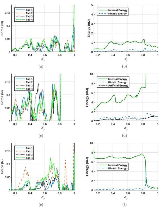
After the unfolding fraction exceeds 0.85, the folds are opened beyond their neutral angle, causing the unfolding forces to increase significantly. D1toD4are tabs used to deploy the packed skin and validate the deployment force and behavior against the experimental data.

Folding GP92 Crease Pattern with Zero-Stiffness Creases in Abaqus/Explicit

Folding with Hub and Facet Rotation

This time was chosen so that the kinetic energy at the end of the folding step was <5% of the internal energy. At the end of the folding stages, stress concentrations of 81 MPa develop at the vertices.

Removing Vertices

The artificial energy builds up to 0.0017 J, or 35% of the internal energy at the end of the folding step. Setting up the GP92 crease model when starting from a folded configuration is still performed with Abaqus/Explicit in Section 3.9.

Figure 3.9: Von Mises stresses within the creased thin-film sheet during folding in Abaqus/Explicit.

Folding GP92 Crease Pattern with Zero-Stiffness Creases in LS-Dyna

Folding with Forces

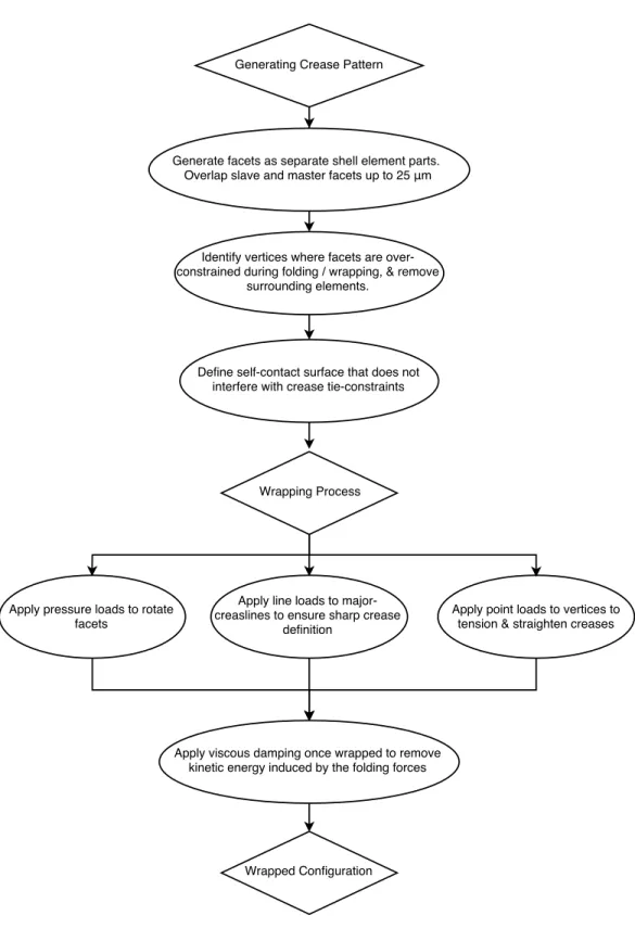
When folded with simply compressive and line loads, however, the main crease line bordering the triangular side is under compressive loads of -5 MPa. To clearly show the crease line between the triangular and quadrilateral faces, the individual faces are shown in separate colors and the center is hidden for clarity.

Figure 3.17: Schematic of a creased surface being folded by point, line and pressure loads.

Including Mass Nodal Damping and Vertex Forces

The compression in the triangular facets and the high tensile stresses in the first ring of quadrilateral facets are caused by the innermost facets being overly constrained during folding. In Section 3.9, this model is validated by comparing the required insertion force in the simulation with the experimental results in Figure 3.4.

MCFF Modeling Technique

Advantages

The moment-angle relationship for each fold need not be determined prior to modeling the packed state. Lack of rotation boundary conditions ensures that exact rotation vectors and angles do not need to be determined.

Figure 3.23: MCFF algorithmic approach to model the folding of creased sheets in LS-Dyna.

Disadvantages

Validation of Modeling Techniques

Analytical Approximation of the Folded Configuration

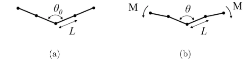
To avoid initial contact between tightly packed layers in FEA software, a nonzero initial fold angle θ0 is required, as shown in Figure 3.25. The minimum θ0 depends on the film thickness and the length of the elements adjacent to the crease L. 3.8) The initially folded configuration as implemented in LS-Dyna is shown in Figure 3.26.

Deployment Simulations

Rather than completely controlling the boundary conditions on the edge of the GP92 folding pattern, the deployment tabs allow the structure to jump from one equilibrium configuration to another, larger radius one. To determine the effect of the MCFF approach, a deployment stage was added to the package.

Figure 3.26: LS-Dyna model of the GP92 crease pattern when starting from an initially folded configuration

GP92 Deployment Results

Mesh Convergence Study

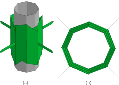
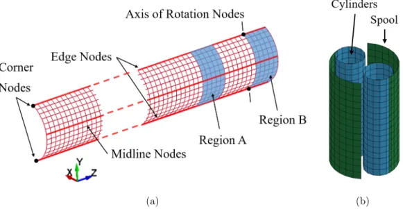
During wrapping, the nodes labeled Diin Figure 3.6 were moved radially inward with boundary conditions during wrapping to completely control their position and ensure that the lobes remained slack. The lobes were modeled as membranes to prevent the lobe bending stiffness from disturbing the rotational symmetry during folding.

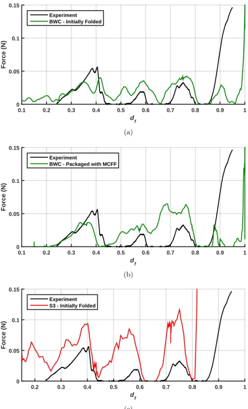
Comparison of Initially Folded and Initially Flat Results

The force increases drastically at df = 0.8 due to indentations occurring in the triangular facet mesh closest to the hub. In contrast to the originally folded LS-Dyna simulation, the force reaches zero at df = 0.44, showing a true equilibrium configuration.

Figure 3.29: Comparing LS-Dyna deployment force profiles for BWC and C 0 shell elements for (a) the initially folded case and (b) packaged via MCFF technique, and comparing Abaqus/Explicit deployment force profiles for S3 shell elements for the initially f

Discussion

The radial force on each tab required to deploy the wrapped GP92 fold pattern is plotted in Figure 3.31 for the LS-Dyna and Abaqus simulations. For the Abaqus simulation, artificial energy builds up until it is 7% of the internal energy at df = 0.8.

Figure 3.31: Smoothed radial force data (left) required to deploy crease pattern and the cor- cor-responding energy (right)

Summary

Analytical models already exist for the unfolding of a tape spring with a single localized fold, and the unfolding of a tape spring from around a hub Rhub ≈ Ri [45], see Sections 2.4.3 and 2.4.4 for details. In Section 4.1 the most suitable elements for modeling the dynamic unfolding of a ribbon spring are determined, while in Section 4.2 different damping techniques are used to match experimentally observed energy absorption.

Unfolding Dynamics of Tape Spring with a Single Fold

Computation of Folded Configuration

The flattened boundary conditions were relaxed and the tip of the band spring was moved so that the band spring wrapped around the cylinder. The term (l0−Rhubθ) corresponds to the free length of the strip spring that is not wrapped around the cylinder.

Figure 4.2: Regions of the tape spring to which boundary conditions are applied during the folding process.

Unfolding Results

In simulations using S/R Hughes-Liu shells, the localized fold traveled 60 mm down the strip spring before stopping. Consequently, the localized fold travels up the strip spring at a lower speed than before the reflection.

Figure 4.5: Isometric view of the folding process (a) Flattening tape spring, (b) Adding contact with folding cylinders to form localized fold, (c) Final folded configuration.

Effect of Energy Absorption on Unfolding Dynamics

Non-Reflecting Boundary Conditions

LS-Dyna models far-field effects by providing non-reflective boundary conditions which can be applied on a single face to certain solid elements. Non-reflective boundary conditions have very little effect on the behavior of the meshed strip spring with fully integrated quadrilateral shell elements.

Viscous Damping

Figure 4.11(a) shows the reflective boundary conditions applied to the bottom only (RB1) and applied to both the bottom and the sides in Figure 4.11(b) (RB2). The second effect is to increase the time it takes for the localized fold to travel along the tape spring.

Coiling and Dynamic Uncoiling of Tape Springs

Coiling

During this step, the corners of the free end of the tape spring are constrained to move only tangentially to the coil. The purpose of this step is to reduce the curvature of the tape spring where it enters the coil.

Figure 4.14: Isometric views of (a) tape spring, including node sets and regions where boundary conditions are applied, and (b) the central hub

Dynamic Uncoiling

For each of the following LS-Dyna settlement simulations, the initial λ0 was measured and inserted into equation 4.4.

Figure 4.17: Snapshots of the uncoiling of tape spring wrapped in opposite sense, meshed with fully integrated LS-Dyna (Type -16), quadrilateral shell elements from around a fixed spool

Discussion

Ri is the final longitudinal bend radius and Rt is the initial transverse radius of the tire spring. The blue line corresponds to the hub and the red line to the starting configuration of the ribbon spring.

Figure 5.1: Schematic of a tape spring folded around a cylindrical hub of radius R h

Opposite Sense Wrapping Experiment with R hub = 4.125R i

Tape Spring Properties
Experimental Setup
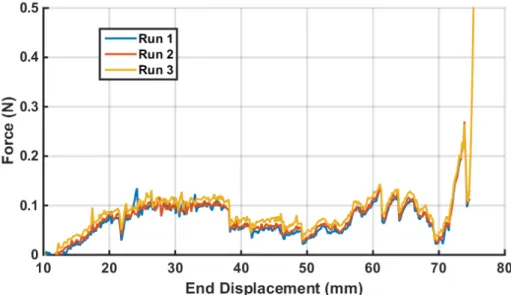
Measuring the Friction Coefficient
Wrapping Experimental Results

The strip spring was folded around the center creating two localized folds, and the non-pinched end was attached to the loading beam of an Instron tensile testing machine. Before performing the winding experiment, it was important to measure the coefficient of kinetic friction between the tape spring and the spreader.

Figure 5.4: Experimental setup for wrapping a tape spring around a hub of radius R hub = 4.125R i

Comparison with LS-Dyna Simulation

Folding Steps
Wrapping Simulation Mesh Sensitivity
Sensitivity to Mass Nodal Damping
Localized Fold Bifurcation
Higher Fidelity Wrapping Simulation
Fully Wrapped Configuration

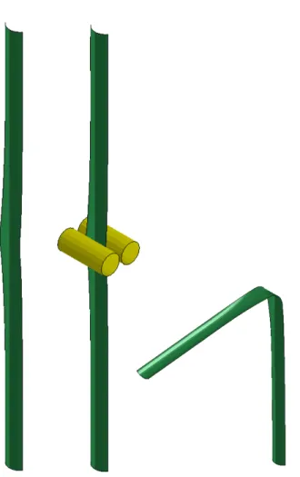
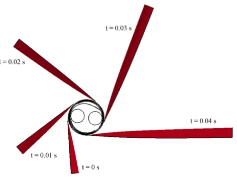
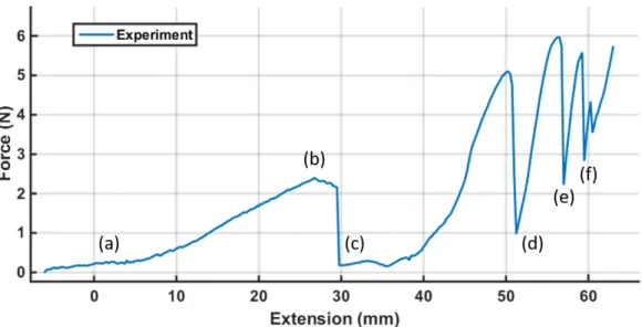
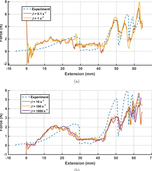
The simulation started with the tape spring in the fully deployed configuration, as shown in Figure 5.8(a). The force profiles for the winding of the band spring for β = 1 s−1 and 10 s−1 are compared with the experiment in Figure 5.11.

Figure 5.6: Force profile corresponding to the opposite-sense wrapping of a steel tape spring around a steel hub, where R hub = 4.125R i

Effect of Hub Radius on Tension Force

Results

The force required to wrap a tape spring around a center 0.4Ri ≤Rhub ≤0.7Ri is shown in Figure 5.19. For ratios 0.7Ri ≤ Rhub ≤ Ri, the exact tension force when the strip spring is fully coiled was difficult to obtain from the force versus displacement profiles.

Figure 5.19: (a) Tension force required to fully wrap the steel tape spring for 0.4R i < R hub < 0.65R i

Extension to Non-Isotropic Tape Springs

At the end of the displacement of dend = 12.5 mm, the spring area of the strip between the two folds comes into contact with the spreader. Then the point of contact between the bar spring and the center slides along the surface of the distributor.

LS-Dyna Simulations

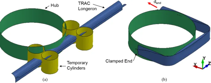
As the dent increases in size in the dual configuration, the point of contact between the hub and the tire spring moves around the hub. In the second simulation, the actual cross-sectional dimensions were varied along the length of the ribbon spring, as shown in Figure 5.21(b).

Figure 5.23: Force profiles corresponding to opposite-sense wrapping experiments of an ultra-thin carbon fiber tape spring around a steel hub.

Discussion

Localized Bend Radius
Simplified Version of Localized Bend Equation
Numerical Analysis of Coiling Behavior

Folding Step
Coiling Results

Coiling Experiments
Capturing Imperfections in Boom Geometry

The effect of the number of localized folds is evident in the corresponding power plots. In the triple initial configuration, the inner flange contacts the hub in two places and the resulting plateau is at 0.1 N. The double initial configuration is closest to that modeled in LS-Dyna.

Figure 6.1: (a) Initial configuration of coiling numerical simulation. (b) boom folded with two localized bends and temporary cylinders removed

Unwrapping and Re-wrapping

Simulated Coiled Configuration

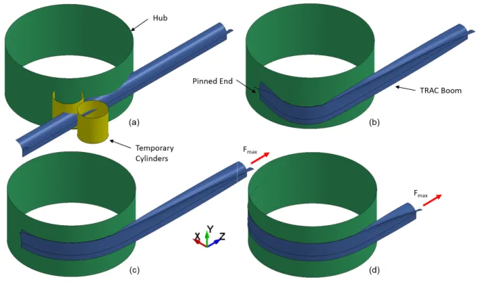
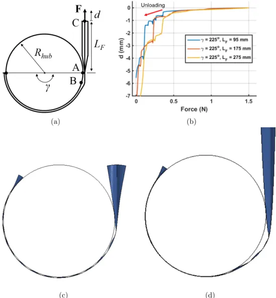
A tension force Fmax was then applied to the end of the boom, causing the boom to coil tightly around a 90o arc around the hub, as shown in Figure 6.9(c). The length of the boom extended and the wrapped angle were found to be the most important factors.

Effect of Uncoiled Length on Unloading

Finally, the center and fixed end of the TRAC boom were rotated about the hub axis, resulting in the coiled configuration of Figure 6.9(d). The effect on the decay force of the simulation time, the magnitude of Fmax, the type of end boundary condition, the length of the unwrapped boom and the wrapped angle were investigated.

Figure 6.9: (a) Initial configuration of coiling simulation. (b) Boom folded with single localized bends and temporary cylinders removed

Unloading & Re-Loading Coiled Boom

This behavior is caused by the normal force on the hub from the inner flange at point A. ForLF = 95 mm, point deflection caused by the localized fold opening occurs until the force drops to 0.12 N, then the sudden deflection change is caused by the inner flange opening in a global sense.

Discussion

As the free length increases, the flange at point A can be opened further for a given tension force F. During unloading, the localized bend where the free end meets the distributor increases in size.

Figure 6.10: (a) Schematic of coiled boom, (b) Force vs tips deflection for unloading curve when controlling γ and varying free length L F

Tape Springs and TRAC Booms

Future Work

In 52nd AIAA/ASME/ASCE/AHS/ASC Structures, Structural Dynamics and Materials 19th AIAA/ASME/AHS Adaptive Structures Conference (April 2011), p. Proceeding of 52nd AIAA/ASME/ASCE/AHS/ASC Structures, Structural Dynamics, and Materials Conference (2011), p.

Figure A.4 shows the viscous damping profile applied to remove the kinetic energy once the sheet was fully folded

Effect of Varying Mass Nodal Damping

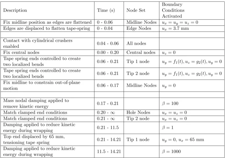
Section B.1 contains the boundary conditions and the corresponding figure showing the sets of nodes for the simulations detailed in Section 5.3. The boundary conditions for the wrapping simulation in Section 5.3 are detailed in Table B.1, and the corresponding sets of nodes are defined in Figure B.1.

Table B.1: Boundary conditions for the simulation in Section 5.3. f 1 (t), f 2 (t), g 1 (t), g 2 (t) were calculated with Equation 4.2

Effect of Varying Friction Coefficient

In addition, for µ≥0.19 the third bifurcation occurs later, at dend = 55 mm, without the sharp drop in tension force at df = 0.51 mm observed experimentally or for simulations with lower friction coefficients.

Figure B.2: Comparison of experimental results and simulation results with mass nodal damping set to (a) β = 0.1 − 1 s −1 and (b) β = 10 − 1000 s −1 for the entire wrapping simulation

Effect of Meshing with Fully Integrated Quadrilateral Shells

The boundary conditions for the wrapping simulation in Section 6.2 are described in detail in Table C.2 and the corresponding node sets defined in Figure C.1. The tension force profile applied to the TRAC boom during coiling, unloading and reloading is shown in Figure C.2.