Antenna-mediated Airspeed Feedback in the Control of Flight Dynamics in Fruit Flies and Robotics
Thesis by
Sawyer Buckminster Fuller
In Partial Fulllment of the Requirements for the Degree of
Doctor of Philosophy
California Institute of Technology Pasadena, California
2011
(Submitted May 26, 2011)
c 2011
Sawyer Buckminster Fuller All Rights Reserved
To Mom.
The key to a good thesis, I am convinced, is a well-selected opening quote.
- S. B. Fuller
Acknowledgments
Extreme thanks to Richard Murray for bringing me in, and for probably being my favorite advisor ever, and I've had a few. Thanks for letting me start on a great project, giving me exibility to move around (and start working with ies), and pretty much everything else you could ask for, including saying how great my work is. To Michael Dickinson for letting me work on a crazy idea. To Joel Burdick for bringing me into Caltech. To Andrew Straw for getting me started thinking about correlators in the rst place and for showing me how to do software the open-source way. This includes lots of tweaks on his software for my purposes, and for writing software good enough to do do things like measuring fast gust responses within milliseconds continuously for 24 hours. His software pervades this thesis. To Linda Scott for always having a smile. To Anissa Scott, Gloria Bain, Lilian Porter for making things all work. Thanks to colleagues and friends who were helpful sounding boards or gave invaluable feedback or just had a kind word, Akira Mamiya, Andrea Censi, Jasper Simon, Shuo Han, Dionysios Barmpoutis, John Dabiri, Ufuk Topcu, Elisa Franco, Ros Sayaman, Alice Robie, Will Dickson, Manuj Swaroop, David Gleason, Erik Schomburg, Jerry Cruz, Pratyush Tiwary, David Brown, Pelayo Dominguez, Aron Varga, Jessica Bastiaansen, Costas Anastassious, Celia Shiau, Olivier Delaire. And thanks Mom who always knew what to say when I was stuck somewhere in my work and knowing I could build great things, and to Dad for showing me how to build them.
Abstract
Achieving agile autonomous ight by an insect-sized micro aerial vehicle (MAV) will require improved technology that is radically smaller, lighter, and more power-ecient. One animal that has solved the problem is the y, a virtuoso among insect yers whose nervous system can perform sophisticated aerial maneuvers under severe computational constraints. This thesis is concerned with understanding and emulating the dynamics of the y's feedback control system. Because vision is noisy and information rich, processing time may a problem for a fast-moving MAV or y. By tracking the fruit y Drosophila melanogaster in free ight in gusts of wind, I found that they incorporate feedback from wind-sensing antennae in a fast feedback loop that dampens the forward-ight dynamics. The slower dynamics are easier to control for long-delay visual feedback, making the y more robust to the limitations of its visual system. Using the y as inspiration, I designed a minimal, visual autocorrelation based controller that used a small array of visual sensors to stabilize a fan-actuated hovercraft robot in a narrow corridor. Using a model for correlators developed for the robot, I showed that a uniform array of visual correlators was sucient to explain the free-ight velocity regulation behavior of ies, rather than a dierent model. In addition to illustrating the benets of concurrent scientic analysis and engineering synthesis, the results give new insight into how to control small biological and man-made ying vehicles using limited, noisy sensors.
Contents
Acknowledgments v
Abstract vi
1 Introduction 1
2 Responses of Free-ight Flies to Gusts of Wind 6
2.1 Abstract . . . 6
2.2 Introduction . . . 6
2.3 Methods and apparatus . . . 10
2.3.1 Realtime y tracker . . . 10
2.3.2 Wind gusting . . . 10
2.3.3 Visual stimulus . . . 13
2.3.4 Flies . . . 13
2.3.5 Trial protocol . . . 14
2.4 Results . . . 15
2.4.1 The groundspeed of ies without aristae is highly variable . . . 15
2.4.2 A long time delay in the visual response could explain the variability . 17 2.4.3 The antennae response is much faster, suggesting a stabilization mech- anism . . . 17
2.5 Conclusion . . . 19
3 System Identication of the Fly's Visual and Mechanosensory Feedback Controller 21 3.1 Abstract . . . 21
3.2 Introduction . . . 21
3.3 Methods . . . 22
3.4 Wing damping . . . 25
3.5 Antennae model . . . 26
3.6 Visual model . . . 30
3.7 Sensory Fusion . . . 33
3.8 Predictions of the model . . . 35
3.9 Discussion . . . 37
3.9.1 The gust response paradox . . . 40
3.9.2 Remarks on feedback architecture . . . 40
3.9.3 Relation to previous work . . . 42
3.9.4 Mechanisms . . . 43
3.9.5 Robustness to variability . . . 44
3.9.6 Robustness to environment geometry . . . 44
3.10 Appendix: Parameters used in simulations . . . 44
4 An Insect-inspired Autocorrelation Model for Visual Flight Control in a Corridor 48 4.1 Abstract . . . 48
4.2 Introduction . . . 48
4.3 Insect Flight Control . . . 51
4.4 Frequency-Domain Analysis of Correlators . . . 52
4.4.1 Correlator response to panoramic image motion . . . 52
4.4.2 Decomposing correlator response . . . 52
4.4.3 Incorporating the eect of spatial blurring . . . 53
4.4.4 Incorporating motion parallax and perspective . . . 54
4.5 A Controller That Uses Correlators to Approximate Retinal Velocity . . . 56
4.5.1 Tuning σ and ∆φ angles for the environment to approximate retinal velocityνr . . . 57
4.5.2 Implementation in simulation . . . 58
4.6 Robotic Implementation . . . 59
4.7 A Controller Designed for Correlators . . . 63
4.7.1 Approximations to correlator model . . . 63
4.7.1.1 Aliasing factor (Equation 4.13) . . . 64
4.7.1.2 Temporal factor (Equation 4.12) . . . 64
4.7.1.3 Perspective approximation . . . 64
4.7.2 Finding state variables by square harmonics . . . 65
4.8 Conclusions and Future Work . . . 67
5 How Flies Use Correlators to Control Forward Velocity 70 5.1 Introduction . . . 70
5.2 Methods . . . 73
5.2.1 Model . . . 73
5.2.2 Drum case . . . 74
5.2.3 Tunnel case . . . 74
5.2.4 Apparatus . . . 76
5.2.5 Simulation . . . 77
5.3 Results . . . 79
5.3.1 Data . . . 79
5.3.2 Model tting . . . 83
5.3.3 Velocity sensing . . . 85
5.4 Discussion . . . 86
6 Conclusion 89
Bibliography 93
List of Figures
1.1 Feedback and control block diagram of the y . . . 4
2.1 Multimodal sensory input to the y . . . 8
2.2 Diagram of experimental apparatus. . . 11
2.3 Photographs of the free-ight tracking and wind gusting apparatuses . . . 12
2.4 Flies ying without their aristae are unstable, possibly because of a long delay in visual feedback . . . 16
2.5 Flies' antenna-mediated response to wind gusts is much faster than their visual response and could eliminate the oscillations observed in arista-less ies. . . . 18
2.6 A hypothesis for how antennae could act to reduce oscillations. . . 19
3.1 A diagram of how tunnel-frame inputs and outputs are transformed into y- frame inputs and outputs. . . 23
3.2 Aerodynamic wing drag is roughly proportional to airspeed. . . 27
3.3 System identication supports a proportional controller with a 20 ms delay as the antennae feedback controller. . . 29
3.4 A good t for the visual controller is an integral controller with a 60 ms time delay . . . 32
3.5 Vision and antennae response forces combine by summing . . . 34
3.6 Addition of the eect of the antennae wind sense increases performance and robustness, with a small cost of increased susceptibility to wind gusts at inter- mediate frequencies . . . 36
3.7 Comparison of response of model compared to data in the velocity domain . . . 38
3.8 Step response of the velocity-domain model reported in other work to our model 39 3.9 How distance to obstacles aects gain in the visual feedback loop . . . 45
3.10 Block diagram of feedback system, rearranged for ease of analysis . . . 47
4.1 Diagram of the correlator. . . 49
4.2 Diagram of fan-actuated robot with array of correlators in a corridor. . . 50
4.3 Simulated and analytic model correlator response R for dierent visual sensor blurring widths σ. . . 55
4.4 Simulation of robot using Humbert controller (sinusoid harmonics) and tuned blur width σ and correlator distance∆φ. . . 59
4.5 Diagram of the fan-actuated hovercraft robot in its environment . . . 60
4.6 Images of the robot and corridor . . . 61
4.7 The luminance response prole of an individual infrared sensor . . . 62
4.8 Trajectories of the robot in the corridor captured by the overhead vision system 63 4.9 Correlator response to state perturbations as a function of body-frame angleφ0. 65 4.10 The controller introduced in this work, designed explicitly for the correlators, has a larger basin of attraction in simulation and functions on non-sinusoid patterns as well. . . 68
5.1 Photograph of corridor with short-wavelength gratings back-projected onto the walls . . . 76
5.2 Visualization of correlator simulation . . . 78
5.3 Simulated and analytic correlator responses for dierent spatial frequencies . . 79
5.4 Drum ground speed trajectories . . . 80
5.5 Tunnel ground speed trajectories . . . 81
5.6 Fly accelerations in response to visual stimuli exhibit a temporal frequency tuning peak . . . 82
5.7 Model correlator responses to drum and tunnel stimuli . . . 83
5.8 By tuning the blur width in the correlator, it is possible to achieve an agreement between the relative responses at dierent spatial frequencies . . . 84
5.9 Fly acceleration response plotted as a function of velocity . . . 85
5.10 The model predicts that correlators could perform good-enough velocity esti- mation in the range ofFs= 4 to 16 cycles/m in a tunnel geometry . . . 86
6.1 The ight trajectories of the fruit y as they explore in the ight arena, as seen from above. Each dot is scaled according to ight speed, as if the animal was dribbling paint as it was ying. The stars indicate when the ies were subjected to a rapid gust of wind. Can we explain this complicated behavior? 92
List of Tables
3.1 Fit values for candidate antenna controllers . . . 46 3.2 Fit values for candidate visual controllers . . . 46 3.3 Parameters used in simulation . . . 46 5.1 Simulation parameters for model of y's forward-velocity correlator-based ve-
locity controller . . . 83
Chapter 1
Introduction
Man has always aspired to y. But only very recently in history has he begun to do so, starting with the Wright Brother's rst faltering ight in an airplane. Man-made craft have since left the atmosphere and even brought humans to the moon and rovers to Mars. But while the past century of ight innovation can be marked by milestones of bigger and faster, from the advent of jet power to supersonic ight to rocketry, today the focus of innovation has changed. New milestones are being measured by smallness, autonomy, and complexity [1]. Small-scale autonomous ight of a vehicle on the scale of an insect is an unsolved current research question. The diculties are manifold: as sensors are reduced in size, their capability and precision must diminish as components are removed. Simultaneously, the available onboard computation power must use less power, limiting the choice of algorithm [2, 3].
One approach to building a small ying vehicle is to improve technology iteratively, building successively more sophisticated and smaller robots with each new generation by adapting existing technologies for reduced size and weight. In open spaces, small ying airplanes such as the Aerovironment Wasp use the global positioning system (GPS) to navigate between waypoints for military surveillance [1]. But in more conned and cluttered spaces, the problem becomes more dicult. GPS cannot indicate the position of obstacles, and even if the vehicle were equipped with a perfect onboard map of them, both the accuracy and bandwitdth of GPS become insucient to avoid collisions below a certain scale [3].
Indoors, GPS is denied entirely, and other methods must be employed. Shen [4] reports an autonomous quadrotor helicopter that operates indoors without GPS by using a laser rangender and an inertial measurement unit to build a map. As impressive this technical feat, the robot is large, on the order of a meter across, so that it can carry the sensor suite
and powerful processor required. It also moves slowly. As vehicles get smaller, and greater maneuverability is desired, powerful sensors like laser rangenders and computers must be done without because of their weight [2]. While vision can give precise estimates of self- motion, existing algorithms such as the one in use on the Mars rovers are slow computation heavy, requiring minutes for each step on Mars [5]. A new approach is needed [6].
Biology, which excels in the domain of smallness and sophistication, may suggest possible solutions. Hundreds of millions of years of evolution has lead to ies, butteries, humming- birds, all of which are able to perform admirably without fast serial computers or lasers [7]. Their ight capabilities exceed current human-engineered solutions [8], often exploiting unsteady uid ow dynamics in their apping ight [9, 7]. Insects are of particular interest because of their relatively simple nervous systems. Because their neurons are typically spec- ied individually with characteristics that are conserved across individuals and even species [10, 11, 12, 13], it seems that an understanding of how their neurons operate to generate behavior is closer at hand [14, 15] than in vertebrates.
Engineers often take inspiration from biology. The original inspiration for feedback con- trol lay in the term cybernetics, coined by Norbert Wiener to refer to feedback control in biology [16]. An eort to emulate the brains of insects lead to an inuential body of work by Brooks that challenged the foundations of robotic intelligence [17]. Instead a traditional ap- proach to robot control, which modularized sensing, modelling, planning, and execution, he proposed tying sensors directly to actuators [18]. Higher level competence at behaviors like foraging were implemented by adding layers that modulated the lower-level locomotive be- havior, mirroring the evolution of the brain [17]. Though these controllers were implemented on ambulatory and wheeled robots, they were never applied to aerial robots.
Findings about ying insects have been the inspiration for many robotic micro-yers in other groups. Biological inspiration may be particularly valuable in ight, where realtime behavior, minimal computation, and sophisticated motion control are specialties of biological organisms [7]. The nding that bees center their ight in a corridor led to robots that balance lateral optic ow [19, 20, 21, 22]. Later, it was found that the lobula plate tangential cells integrate visual ow over wide-eld patterns corresponding to states of self motion [11, 23, 24] and seem to be required for important insect motor control tasks [11]. This inspired the idea of decomposing visual ow into matched lters for self motion [25, 20, 26], including sinusoid harmonics, from which the state vector of the vehicle can be observed and
controlled [27, 2]. A small airplane inspired by the expansion-avoidance behavior observed in ies [28] was able to y autonomously in a small room by making body-saccades away from walls [29]. A robot that regulates its attitude using ventral optic ow used a simple, insect-inspired controller that reproduces observations that that insects may descend in a headwind and ascend in a tailwind [30], though recent work has called into question whether that mode of ight control is active in ies [31]. Using Hebbian updates to learn and perform visual servoing demonstrates how correlators could arrive spontaneously during learning or evolution [32, 33]. For a review of bio-inspired engineering, particuarly in the domain of visual ight control, see [22].
Insight the other direction, from engineering into biology, often follows an eort in en- gineering synthesis of a biological system. Only then can we perceive the subtleties that invariably arise when a concept is reduced to practice. Braitenburg [34] showed how sim- ple wheeled robots could show life-like behavior and even the illusion of free will by simple interconnections between sensors and motors. But understanding the principles required mentally constructing and running these little robots. Ijspeert [35] showed how regulation of central pattern generators could lead to transitions between swimming and walking gates on a robotic salamander. Biology's strongest trait is perhaps its ability to nd practical and robust solutions. For example, [36] found by implementing a small apping yer that an automotive-like dierential could compensate for wing damage by using a mechanical pivot to automatically ap the other wing farther. Only by constructing the device could he dis- cover that a mechanical linkage could produce robustness that might ordinarily be presumed to arise from neurally-modulated mechanosensory feedback. This may inform future studies on the insect wing motor hinge [37].
It is the opinion of the author that understanding how to autonomously y small vehicles and understanding how ight is performed by insects is best approached by performing engineering and biology simultaneously. In doing so, the benets of both approaches will inspire bigger ideas.
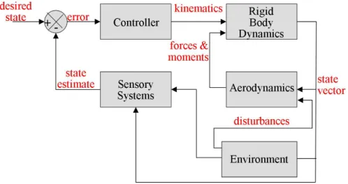
This thesis considers the dynamic ight control of the y from a control-theoretic perspec- tive, an approach that has been lacking in the biological literature [38]. The y's feedback controller is represented as a block diagram, with boxes representing components segregated by function or mechanism (Figure 1.1). I report contributions to the understanding of insect ight control by both studying fruit ies and building a robot that takes inspiration from
Figure 1.1: Feedback and control block diagram of the y. This thesis is concerned with understanding characteristics of the controller and sensory systems blocks.
the y's control system. Fruit ies make a compelling choice for study because of the ease of raising them, the short generation time (9 days), and most importantly, as a genetic model organism, genetic ndings can be leveraged in behavioral studies and vice-versa [14]. In the study of the y, I placed particular emphasis on studying sensory feedback systems that have potential application to robot yers.
The thesis is organized as a series of self-contained chapters, each beginning with an abstract that summarizes the main results and an introduction that reviews the relevant background. chapters 2 and 3 detail how by studying dynamics of forward ight in ies, I uncovered a control challenge encountered by the y that had not previously been addressed in detail: feedback from vision is relatively slow. By subjecting ies to sudden gusts of wind, I made the surprising nding that the antennae act as fast, proportional sensors that act to damp out and thus slow the y's dynamics. The slowed dynamics mitigate the diculty of long visual delays and give the y robustness to variations in parameters ranging from y- to-y variability to environment geometry to non-idealities in visual correlators. And they may be applicable to autonomous ight control, in which computation-heavy vision is likely to be a slow sense as well. Next, I considered ight control from a synthesis perspective in chapter 4. Using a bio-inspired control algorithm with minimal computational requirements, I designed a controller that stabilized the motion a dynamic hovercraft robot using visual
ow estimates arriving from a small array of luminance sensors and correlators. In chapter 5, I found that the analysis of chapter 4 suggested a new study on free-ight behavior in ies to show that basic correlator behavior may be sucient to explain the y's forward speed regulation, rather than necessitating some more complicated model. In addition to illustrating the benets of cross-disciplinary study, the results shed new light onto the ight control of small ying vehicles, biological or man-made.
Chapter 2
Responses of Free-ight Flies to Gusts of Wind
2.1 Abstract
In order to navigate through a complex and changing world, animals must rapidly combine information from sensory channels with dierent response bandwidths and modulate motor output accordingly. For example, to regulate their ight speed, insects are thought to employ both rapid mechanosensory signals and slower visual cues, although the means by which they combine information from these two modalities is unknown. To study this process of sensory-motor integration, we subjected free-ying fruit ies to impulsive gusts, visual gusts, and attenuated mechanosensory feedback by removing the aristae on their antennae. By observing the y's velocity response to wind perturbations, we found that, surprisingly, the fast, antenna-mediated response acted in the same direction as the wind input, in eect augmenting the eect of drag on the wings. Aristae-ablated ies showed much higher variability and oscillations in ight speed, suggesting that the wind sense might not be for wind disturbance rejection but for damping out these ight velocity oscilations.
2.2 Introduction
Flies, among the most adept of insect iers, display a sophisticated suite of aerial behaviors that require rapid sensorimotor processing. They can recover from tumbling surprise take- os in tens of wingbeats [39] and can perform inverted landings on the ceilings with ease.
But even the practical matter of navigating from one place to another in ight is a chal- lenging task requiring sensorymotor specializations. Not only must they negotiate cluttered
environments abounding with obstacles such as trees and plants, but they must do so in wind, which may change direction and magnitude. How this is achieved has not yet been explained, although many clues have been found from studies on ies and other insects.
Flies are visual animals, devoting perhaps two-thirds of the neurons in their brain to visual processing [40]. They have two faceted eyes that sample nearly the entire visual sphere, with varying visual accuity and number of ommatidia depending on species [41, 42]
(Figure 2.1). Insects' ight control relies heavily on visual ow, that is, the pattern of visual motion across the retina. Bees center their ight in a corridor, balancing lateral visual ow, and slow when the corridor narrows [43]. Both of these behaviors are consistent with a regulator that measures the angular velocity of visual ow across the retina (for a review, see [22]). Neurons that average visual motion across the retina have been found in the y brain and homologs of such cells that may underly this behavior [11, 23]. A modeling eort suggests visual motion patterns could be used to orient upwind [44]. Flies also use preferences for simple horizontal or vertical features to structure their ight. They control altitude by keeping level with horizontal features [31] and are attracted to vertical features, using that attraction to y straight and overcome the normally-aversive frontal visual expansion that accompanies forward ight [45]. Flies spend much of their time ying forward and straight.
They organize their trajectories into linear segments of roughly constant velocity, punctuated by sudden turns known as body-saccades [46] that are often induced by visual expansion [28]. Their visual forward ight-speed regulator can be modelled as a delay followed by a second-order velocity controller [47]. A rich literature exists concerning the mechanism of visual motion detection, but evidence suggests that in forward ight, ies' response behavior acts proportionally to the dierence between the y's velocity and the velocity of background visual motion across a range of spatial frequencies [48].
Less well understood is the role played by the antennae (for a review, see [38]). For many ying insects, knowledge about the wind is vital for survival: to nd food sources by smell, a fruit y moves laterally to the wind to search for odor plumes and then turns upwind when one is found [51]. Perhaps the only example of known interaction between vision and wind sensing is that tethered but freely-rotating ies turn into a headwind and then use that percept to overcome the normally-aversive forward visual expansion [52]. Once facing upwind, ies use vision to maintain a constant groundspeed, independent of the speed of wind in a wind tunnel [53, 54].
Figure 2.1: Multimodal sensory input to the y. An electron micrograph of a fruit y's head (top) shows the faceted eyes (red) and the antennae. The eyes take a low-resolution omnidirectional sample of the visual world, which would look something like this computer- generated rendition (below, from [49]). The aristae (top) are branched appendages of the antennae that protrude from the head and deect in wind. Sensors at the base of the antenna, the Johnston's Organ, sense the wind-induced deection [50]. In this and the next chapter, we present a quantitave analysis of the input-output behavior of these two senses simultaneously.
Flies detect wind using sensitive motion sensors in their antennae [55]. The antennae have also been shown to sense sound [56], the direction of gravity [57, 58], and may be directly involved in sensing and controlling wing kinematics [59]. The basic mechanism is that the arista, a branching fourth antennal sement, protrudes into the wind and is subject to a torque roughly proportional to airspeed [50]. The arista, together with the third antennal segment to which it is rigidly attached, can rotate passively around a joint with a roughly vertical axis coincident with the long axis of the third segment. The motion of this joint is sensed by the Johnston's organ, an array of chordotonal mechanosensory organs residing in the second antennal segment. An active antenna-positioning reaction carried out by the rst antennal segment may increase the dynamic range of the wind sense [50].
Evidence suggests that ies can use their antennae to measure absolute airspeed, rather than, for example, its rate of change. In tethered ies, the steady-state wing beat amplitude varies with the steady-state airspeed [50]. Similar observations have been made for locusts [60] and dragonies [61]. More recently, using a calcium-sensitive reporter gene, Johnston's Organ neurons were found to project to dierent portions of the brain depending on whether they responded to either absolute antenna deection or its rate of change [62].
Whereas wing kinematics changes in response to antenna wind stimulation in the the steady-state on tethered animals has been explored, little is known about about how this reaction translates into changes in behavior in free-ight. Because of the range of dierent kinematic motions available to apping insects, it is in general impossible to map changes in wing beat amplitude directly to forces and torques [63, 64]. In addition, tethered kinematics dier signicantly from free-ight kinematics, perhaps because normal feedback signals are disrupted [64]. Hence, it remains unanswered how the documented wing kinematic changes aect ies' free-ight motionsdo they give rise to thrust, lift, or torques, and in what directions? In addition, steady-state analyses do not examine dynamic behavior, which may be key to explaining how these organs aect the dynamic stability of the aloft y.
To investigate the y's sensor dynamics in straight segments of forward ight, we sub- jected them to wind and visual stimuli as they ew along a corridor while their position was tracked by cameras.
We found that the antenna-mediated wind response is much faster than the visually mediated response. But rather than acting to reject the gust of wind as might be expected, the antenna response does just the opposite: the velocity of ies with intact antennae is
more perturbed that for arista-ablated ies. Flies without their aristae showed signicant variance in their forward velocities, nearly twice that of control ies. The variability appears to be sinusoidal, as if the ies are using a along-delay visual feedback loop that is at the edge of stability without the antennae. The antennae reex function may be to act as an active damper, applying force as necessary to dampen these oscillations.
2.3 Methods and apparatus
2.3.1 Realtime y tracker
We used a custom built multi-camera real-time y tracker [65] (Figures 2.2 and 2.3) to record the three-dimensional positions of ies in free-ight. It consisted of ve digital rewire videocameras (Basler A602f) taking images at 100 frames per second, ve dedicated desktop computers performing image analysis to locate ies in each camera's view, and a central computer triangulating that information into (x, y, z) positions. Dimensions of the arena were 150 cm×30 cm×30 cm. Latency was approximately 50 ms. Tracking was performed with infrared backlight and infrared lters on each camera so that moving visual stimuli were not detected by the cameras.
2.3.2 Wind gusting
We constructed two dierent devices to generate sudden changes of wind velocity in the ight arena. The rst was a set of motor-actuated wind-vanes that could open suddenly to allow air pulled by the fan to ow through the tunnel, giving a step input to the y.
Because the arena was in a wind tunnel designed for only uni-directional ow, the fan, and hence the vanes, could produce wind stimuli in only one direction. The second was an air piston that could move the mass of air in the tunnel in either direction very quickly. Though the apparatus was situated behind the y during the trial (Figure 2.2), atmospheric pressure in front of the y provided plenty of pressure to generate headwind gusts. To verify that the timing of the gust was the same along the length of the arena, two wind-measurement probes (described below) were placed 1 m apart at either end and simultaneously measured the gust. The two gust velocity traces were nearly identical with timing dierence of3±1ms, approximately the speed of sound (≈350 m/s). Thus the gust was approximately the same along the length of the tunnel during a single 10 ms frame of the tracking cameras. Both
gust apparatus
(vanes or piston)
free flight arena
+x +y
wind vanes
air piston
local computers camera 1
camera 2 camera 3
camera n 1 2 3 n
central computer
v (projector velocity ) p
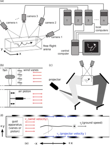
Figure 2.2: Diagram of experimental apparatus. An array of cameras and a cluster of computers processing video images triangulated the position of ies in real-time (a). Wind stimuli (b) were generated either by a fan and wind vanes opening or closing (top) or by an air piston spanning the cross section of the wind tunnel actuated by a linear motor (bottom).
Because the wind tunnel is designed to provide unidirectional laminar ow, the fan could only pull air in one direction. Back-projected visual stimuli were generated by a high-speed monochrome projector reected o of mirrors (c). A diagram of the wind tunnel seen from above (d) shows the locations of the gust apparatus and visual stimuli relative to the y.
In the inertial lab frame, stimuli to the y are wind velocity vw and projector velocityvp. The y's ground speed vg is measured by the tracker as the output. A trial starts when a y passes through the imaginary plane shown as a dotted line transverse to the axis of the wind tunnel. A drawing of an accepted trajectory in which the y ew primarily along the axis of the tunnel is shown as a solid line; a rejected trajectory is shown as a dotted line. All velocities in the tunnel frame have the convention that positive is toward the right, according to (e).
Figure 2.3: Photographs of the free-ight tracking (top) and wind gusting apparatuses (bottom). The free-ight arena is shown in light (top left) and under the experimental conditions of darnkess (top right). The pink glow on the right is the infrared backlighting used by the infrared-only tracking cameras, not visible to either human y eyes, but detected by the CCD sensor in the digital camera used to take the picture.
gusting devices were actuated by a high-speed brushless linear motor (LinMot, Elkhorn, Wisconsin), and could perform short motions in as little as 35 ms or with a distance up to 125 mm. Because the motor servo controller could be programmed with only one trajectory at a time, a given population of ies in the tunnel was subjected to only one type of wind gust for the 24 hour period. The mechanism was commanded to gust by a single voltage pulse from a computer based on the real-time position estimate. The two devices are shown in Figures 2.2 and 2.3.
To minimize visual impact of piston or vanes motion, they were constructed from clear plexiglass and placed so that they were behind the y during each trial. To test whether their motion could induce a visual response, a sham piston with holes spanning most of its cross section that did not generate any measurable wind disturbance when it moved was substituted for the real piston. When tested with ies, there was no discernible behavioral dierence between trials in which the piston was moved and when it was not. This was expected because the physical motion of the gusting apparatus lay entirely in the rearward section of the visual sphere not sampled by the y's eyes [66].
Using a hotwire anemometer (MiniCTA with p55 probe, Dantec Dynamics, Holtsville, NY), the time-course of the gust was measured at 1 kHz. Gusts were repeatable to within 0.02 m/s. The thickness of the boundary layer in the airow in continuous-wind experiments was found to be less than 2 cm, so any trajectories passing within that distance of the walls were eliminated from consideration.
2.3.3 Visual stimulus
Visual stimuli were generated using the Vision Egg software on a PC running Ubuntu Linux with an nVidia Geforce 8500 GT graphics card [67]. A Lightspeed Designs DepthQ projector with color lter wheel removed was used to back-project the patterns (120 Hz update rate), and the mean luminance of the arena walls and oor when the projector displayed midgray was 50 cd/m2. The visual stimuli were sinusoid gratings on both walls with a spatial wavelength of 12 cm, moving in the x-direction. The 12 cm wavelength exhibited a strong response that was found to be roughly proportinal to forward velocity (Figure 5.6). This computer received 3-D coordinate estimates for all ies from the tracking computer over ethernet and orchestrated the automated experiment protocol. Because the visual frame rate of 120 Hz diered from the tracking frame rate of 100 Hz, the position of the visual stimulus was linearly interpolated to the time stamps of the camera frames.
2.3.4 Flies
Flies were 23 day old female Drosophila melanogaster Meigen descended from 200 wild- caught female specimens. Flies were manipulated on a cold stage under a dissection micro- scope. For aristae-ablated experiments, the aristae were removed using sharpened tweezers.
Flies were kept on a 12h:12h light:dark cycle and experiments were started 59 hours before the end of their subjective day, continuing for 24 hours with 10 to 12 ies in the arena at a time. They were starved with water for 4-8 hours prior to each experiment to increase exploratory behavior. Yield was approximately 30 acceptable trajectories/day for control ies, and 15/day for arista-ablated ies. The mass of ies averaged 1.1 mg at the start of trials. After a 24 hour trial period, ies were recovered from the tunnel using a vacuum and were found to have lost approximately 20% of their mass, so the average y mass m was estimated at 1.0 mg.
2.3.5 Trial protocol
A visual connement protocol similar to that described in [48] was used to bring ies to the trigger plane at relatively high frequency, increasing experimental throughput. However, it was not possible to include a plume of odor because the air piston covered the entire cross section of the tunnel, blocking continuous ow. Because of ies' tendency to only y in the presence of a headwind, it was necessary to have them ying forward in the quiescent air at the start of each trial (rather than be stationary but ying into continuous wind, as in [48]).
The protocol used to bring ies to the trigger plane was executed as follows: (1) The walls were animated with velocity in the negative-xdirection to induce any ying ies to move in that direction as well. (2) Once the chosen y (the y with the longest current trajectory) passed a threshold 5 cm away from the trigger plane, the animation direction was reversed again. (3) With animation now in the forward direction, the y was brought forward until it passed the trigger plane. If either of the previous steps did not complete within 2.5 seconds, the protocol returned to step 1. Otherwise, once the y passed the trigger plane, 4) a 1.2- second trial was initiated, consisting of a gust, a visual gust, or a combination of the two, in random order. At the end of this period, the state of execution was returned to step 1.
Because the linear motor interface was written in closed-source software, it could not be programmed and only one piston stroke type was available per population of ies and 24-hour period.
We eliminated trajectories in which ies performed sudden body-saccades, selecting only trajectories in which the y ew essentially along the axis of the tunnel. Trajectories with non-axial velocity magnitudes that exceeded 0.25 m/s (after being ltered by a 10-sample box lter to eliminate transients) were eliminated from consideration. To insure uniform visual stimulus, trajectories not starting in the middle 1/3 (width-wise) of the tunnel were eliminated. Traverse measurements taken with the hotwire anemometer indicated that wind tunnel air ow was uniform farther than 2cm from the walls. Accordingly, trajectories in the upper 2/3 of the arena were accepted, with the exception of trajectories that came within 2 cm of the arena ceiling.
The y tracker records trajectories and performs data association using a nonlinear extended Kalman lter that estimates velocities as well as positions. In parallel, it also estimates positions directly each time step using a least-squares estimate based on projection
onto the rays cast into each camera currently imaging the y [65]. We used this noisier, unltered format because it provided the highest time-resolution, a necessity because of the high-speed dynamics in this study.
Registering the timing of all devices was of key importance. To collect the exact time that each frame from the cameras was taken, the tracking computer used feedback from the camera trigger device to create a model of oset and skew of pulses relative to time information collected over internet from NPT to collect timestamp of each frame. For the timing of the gust, the voltage pulse that induced the gust was recorded along with the wind velocity of the gust so that the timing of the gust relative to the pulse was recorded. The pulse was generated by the same usb trigger device that triggered each frame of the cameras.
The device returned an acknowledgement of the command, and the middle of the roundtrip time (almost aways around 3 ms, and if longer, the trajectory was elimininated) was taken as when gust was started. To time the projector latency, we used a Texas Instruments opt101 light sensor sensor aimed at the projector and the camera trigger hardware to send a voltage pulse so that both could be observed on an oscilloscope simultaneously to nd that the projector had a consistent 20 ms latency. Adjustments for these delays were made in the data post facto.
2.4 Results
2.4.1 The groundspeed of ies without aristae is highly variable
In comparison to control ies with intact antennae, ies with their aristae removed exhibited more variable trajectories and velocities. The variance of groundspeed within-trajectory was greater (4.6 cm/s vs 7.5 cm/s), as was the variance in mean velocities (7.1 cm/s vs 9.9 cm/s) (Figure 2.4). The velocity variability appears to be a result of greater degree of oscillations: ies without their aristae appear to be continually accelerating and decelerating in a sinusoidal pattern.
(a)
(b)
(c)
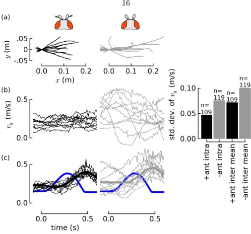
Figure 2.4: Flies ying without their aristae are unstable, possibly because of a long delay in visual feedback. Compared to the trajectories of contol ies with their antennae intact (a, left in black), a random sample of ten trajectories from ies with their aristae removed show (right, in grey) more variability. Trajectories were rendered as seen from above with (0,0) being the y's position at the start of the trial. Arista-ablated ies exhibit more variable groundspeeds (b) that appear to be sinusoid-like. The variability (measured by standard deviation) of velocities of arista-ablated is higher within each trajectory, as the variability in mean velocities, compared to control ies (b, far right). When subjected to a visual stimulus provided by a change in projector speed at the start of the trial, shown in blue (c), ies respond by accelerating, but with a≈100 ms delay. The visual delay could account for the velocity oscillations. Assuming feedback from the antennae is faster than that of the eyes, a parsimonious explanation is that the ies approach instability when forced to rely solely on longer-delay visual feedback alone.
2.4.2 A long time delay in the visual response could explain the variability When subjected to a visual stimulus provided by a change in projector speed, ies respond by accelerating in a way that eliminated the visual slip, but with a delay of ≈100 ms. The visual delay could account for the velocity oscillations. If the feedback system had to only rely on slower-response visual feedback, it could be operating closer to the edge of stability, which would predict larger oscillations arising from the feedback, as can be observed in traces in Figure 2.4 (b).
2.4.3 The antennae response is much faster, suggesting a stabilization mechanism
We measured the groundspeeds of ies in a series of trials with dierent headwind gusts (Figure 2.5). In slow, step-like changes in wind velocity generated by suddenly opening the wind vanes, ies rst decelerated and then recovered their initial velocity after 400-500 ms, consistent with the steady-state behavior rst documented by [54] that ies maintain groundspeed independent of wind velocity. Further, we veried that this behavior was mediated by vision by animating the walls at the same time as the onset of the gust in such a way that the mean visual stimulus during the trial was near zero. Under this condition, ies decelerated to a new velocity and therafter maintained that velocity. A signicant dierence in responses between control and visually-abolished step gust responses only appeared after 200 ms, reinforcing the nding that vision operates with a relatively slow response.
In a fast impulsive gust, unlike in a step gust, an animal moving purely passively with no feedback (with a xed amount of forward thrust to counteract the eect of aerodynamic drag on the wings) would recover its initial velocity after a short time because the wind velocity itself also returns to zero. However, in fast impulsive gusts generated by the air piston (15 mm gusts in 35 ms), we found a signicant dierence in velocity between ies with and without their aristae at 75 ms (Mann-Whitney U-test, p < .001). The divergence appears very fast, within 20 ms. These result suggest that ies sense rapid changes in airspeed with their antennae and respond by actively accelerating in the same direction as the gust. In the gentle, step gusts, the eect is so subtle it is hard to detect.
(a)
(b) + visual stimulus- visual stimulus
gentle step gust strong impulse gust
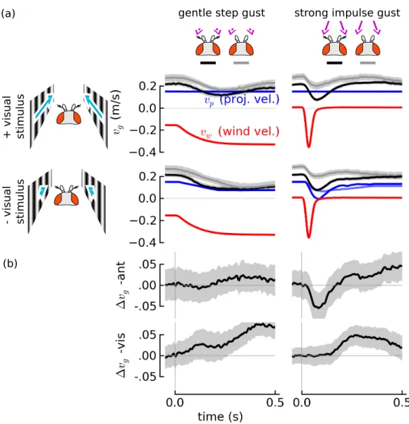
Figure 2.5: Flies' antenna-mediated response to wind gusts is much faster than their visual response. Fly groundspeedsvg (mean +/- 95% condence interval of mean) in gentle, step gusts (a, left) and strong, impulsive gusts (a, right) are compared against the groundspeeds of ies with their aristae removed (gray). In gentle step gusts (left), ies eventually recovered their initial velocity in spite of the increased headwind (upper left), This behavior is most likely mediated by vision. During a headwind gust, the y's velocity drops, inducing visual slip in the negative direction, shown by the blue arrows on either side of a cartoon of the y's head. To eliminate the visual slip normally associated with the headwind gust, the walls were animated at roughly equal velocity to the y's mean velocity (collected from an earlier set of trials) (lower row). With visual animation, groundspeed recovery in the step gusts was abolished (lower left). In strong gusts there is a signicant behavioral dierence between ies with and without their aristae that arises soon after the gust (b, top right). But visual responses take much longer to occur (b, bottom right), supporting the hypothesis that there is a long visual delay. The antenna play and active role in forward velocity regulation and rather than acting to reject the gust, the response seems to abet the eect of the gust.
f (control force)c
v (groundspeed) g
time
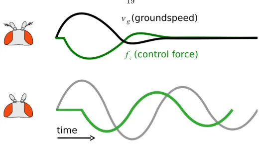
Figure 2.6: A hypothesis for how antennae could act to reduce oscillations. The time it takes for a y to sense that its velocity is dierent from its desired forward velocity and exert a thrust force response fc to eliminate the error (green) is much faster if the y's antennae are intact (top). If instead there is only visual feedback (bottom), the response is so delayed that it leads to a continuation of the oscillations.
What use could there be to actively augmenting the disturbance caused by a gust of wind? The direction of the response from the antennae is in the same direction as would be required to abolish the ground speed oscillations observed in aristae-less ies in Figure 2.4.
A representative diagram is provided in Figure 2.6.
2.5 Conclusion
In this chapter, we presented an apparatus to provide wind and visual stimuli to the fruit y as it ew and its position in space was tracked. We found that the antenna-mediated wind sense is much faster than the visual sense. The direction of the response, however, was unexpected: rather than sensing the wind so that its inuence could be rejected, the antennae appear to be augmenting the passive drag force on the wings with active changes in wing motions. We hypothesized that the function could be to counteract, and thus damp out the oscillations observed in arista-less ies. These ies may be oscillating because they are forced to rely only on long-delay visual information and thus are operating at the edge of stability.
In the following chapter, we describe how a quantitative system identication procedure was applied to nd a model for the y's input-output behavior. We used the model to explain how the antennae function as airspeed dampers, and how this could be used to
provide robustness to parameter variability.
Chapter 3
System Identication of the Fly's
Visual and Mechanosensory Feedback Controller
3.1 Abstract
This chapter concerns a system identication of the y's free-ight behavior in response to wind and visual stimuli. A linear model t to the ies' behavior suggests that the antennae act as a fast, proportional feedback regulator whereas vision provides longer-delay integral feedback, and that the two senses sum. The feedback from the antennae acts to augment the passive air drag of the wings, eectively doubling it, providing a velocity-proportional damper that slows the y's dynamics and makes them easier to control for long-delay visual feedback. Flies without aristae exhibit oscillations in ight velocity that typify a feedback regulator at the edge of stability, as predicted by the model. The additional information provided by airspeed measurement may aid the y in conned visual environments where the eective visual gain depends on the angular rate of motion across the retina which varies greatly depending on the distance to obstacles. Our results provide new insight into the functional architecture of ight control systems in insects.
3.2 Introduction
This chapter succeeds chapter 2 by nding a quantitative model of the y's behavior so that statements can be made about its design and performance. We proposed a number of simple candidate linear models and t them to the y's response to a number of dierent wind and
visual gusts and selected the best model.
We found that the antennae functioned as fast active sensors with a feedback response proportional to airspeed. Since the visual response has a longer delay and hence is slower, the damping of the antennae slows the dynamics and makes forward motion of the y easier to control with visual feedback. This has two interrelated consequences. First, there is less overshoot by ies with intact antennae, and thus velocity oscillation in ies with intact antennae, as shown in Figure 2.4 of the previous chapter. Second, the antenna eect increases robustness to changes in gain or time delay. It takes a much smaller increase in time delay (such as from cold weather or the eects of ethanol) or increase in gain to make a y without aristae unstable with respect to forward velocity control. A number of eects can increase visual gain: odor [68], visual brightness or contrast [69, 70], state of excitation, y-to-y variability, or most importantly, in conned spaces the visual response will be higher for a given speed because of higher angular rate of visual motion across retina [71]. The antennae give the y robustness to limitations in its visual system.
3.3 Methods
Since all inputs and outputs are received in the moving frame of the y, we considered the feedback mechanism from that perspective. Thus neither were the y's inputs directly observed nor its outputs directly measured, but inferred using both information about the y's velocity and tunnel-frame inputs.
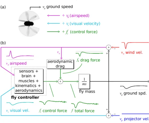
As the y moves, it experiences visual motion on its eyes, which we will call vv for visual velocity. It is necessary as well to dene a direction convention, and so we dened positive to be the direction experienced by the y when it is moving forward, known in the literature as progressive visual motion. We likewise dened positive airspeed va to be in the same direction (Figure 3.1).
ground spd.
vg
total force f
+
va vwwind vel.
vpprojector vel.
visual vel.
vv
Figure 3.1: A diagram of how tunnel-frame inputs and outputs are transformed into y- frame inputs and outputs. The two inputs, visual velocity vv and airspeed va, and one control force output fc are dened as positive along the direction of the arrows (a). A block diagram (b) indicates how tunnel-frame disturbances (right) are transformed into the moving frame of the y, with example traces showing how a wind disturbance would be propagated. The goal is to nd an abstract model of the box labeled y controller. Color conventions introduced for dierent quantities in this gure are used throughout the paper.
In the xed geometry of the arena, we dened the visual velocityvv as a linear term, but the y probably measures angular rate across the retina [43], averaged over portions of the visual sphere. The mechanism for visual motion detection is likely a correlator [72] combined with spatial averaging by tangential cells [73, 23]. More detail is given in the introduction to Chapter 5. That the y is likely measuring angular visual rates has implications for feedback control in varying geometries, to which we will return in the Discussion.
Because the dynamics of the y can not be approximated as primarily viscous in nature at the timescale considered here, we performed modeling in the domain of forces. Previous studies on free-ight forward ight [48, 47] have modeled y visual ight speed response in velocity domain only. But in this work, because the response from the antennae is much
faster, it is necessary to model the dynamics in the force domain. Equating forces and accelerations along the x-axis, the force-balance equation for the y is
fc+fd=mv˙g, (3.1)
wherefc is the active control force generated by the y in response to sensory stimuli and fd is the passive drag force arising from baseline wing kinematics . The y changes its wing kinematics from baseline motions to alter the active force fc, but we do not address the specic changes that occur in this work. Results from [74] indicate that passive wing damping drag force fd is roughly proportional with airspeed va, as do our results and a simulation on an aerodynamic apping-wing fruit y model based on data taken from a dynamically-scaled model in a tow-tank [49] (and see Figure 3.2). A dynamic element with force proportional to velocity is known in control engineering as a dashpot or viscous damper. Call this coecient of proportionality b, so that fd = −bva. If inertial forces dominate (short timescales), the force balance equation (Equation 3.1) reduces tofc=mv˙g, and if viscous forces dominate (longer timescales), then it reduces to fc = bva. The time constant of exponential relaxation to asymptote velocity in response to a steady force in the full force balance equation is equal to mb ≈ .13 s. Considering delay from vision reported in [48] is 0.081 - 0.1 s, the slower velocity-domain viscous dynamics may be sucient for the purposes of purely visual modeling. But the faster antenna response we consider in this work necessitates inertial dynamics so the slower viscous domain dynamics approximation cannot hold.
Moving to the domain of active sensory feedback, we seek a model for both drag and active control forces. But rather than perform an exhaustive search among all possible nonlinear models, we considered a set of simple, plausible linear models. If a satisfactory one could be found, no further analysis would be necessary. And in general if they do not have strong nonlinearities, nonlinear systems can be approximated by linear ones in a large- enough neighborhood around equilibrium. Thus complicated nonlinear spiking ensembles of neurons performing computations in the nervous system of the y may be abstracted as linear. Because the drag was roughly linear, this was considered as further evidence that linear models could be sucient. The tting approach was to perform least-squares ts on each candidate model. For clarity, the results are segregated by functionality into delay and
gain boxes, but most likely both operations are being performed by a single sensory-motor transduction cascade.
To estimate velocities and accelerations from position information, we ltered using causal linear lters and a rst-order hold input model (linear interpolation between input data points). All ltering and tting computations were performed using the python-control package version 0.3 (http://python-control.sourceforge.net/) and SciPy (http://www.scipy.org).
Accelerations were calculated from position using a lter of the form (τ s+1)s2 2, whereas ve- locities were estimated using the lter (τ s+1)s 2. When the information was already in nal form, such as wind velocity measurements from the hotwire anemometer, it too was ltered, but with the lter (τ s+1)1 2 so that any phase lags induced by the ltering were replicated in all data. The time constantτ used in the lters was 3 ms.
3.4 Wing damping
It was rst necessary to nd a relation for the passive drag forces acting on the y. To eliminate antenna feedback, the aristae of ies were removed, and to eliminate visual feed- back, we considered only data coming from the early, pre-visual period of the gust. Based on experiments on tethered Drosophila performed by [74], as well on a quasi-steady model of apping Drosophila wings based on data from a dynamically-scaled tow tank [49], we expected the drag force to be roughly proportional to the airspeed, or fd = −bva. While airspeed drag at the scale of the y would be expected to be primarily inertial, and thus proportional to airspeed squared, this does not take into account the eect of apping wings. Consider this approximation: suppose wing angle trajectory can be aproximated as a sawtooth (rather than a more realistic sinusoid [9]), with va the free-stream airspeed and w the mean velocity of the wings relative to the y, with w va. Then drag on the downstroke (into the wind) is fd= −α(va+w)2 according to the relation for intertial ow drag, whereα incorporates coecients of surface area, coecient of drag, and air vis- cosity. On the upstroke, the drag reverses direction because the wings are moving much faster than the free-stream, and the drag force is fd = α(w−va)2. Since upstroke and downstroke take equal time, the stroke-averaged force is just the average of these two, or fd = 12α(−va2−2vaw−w2+va2−2vaw+w2) = −2αvaw. Thus the drag on the apping wings is proportional to va assuming w is constant (assuming negligible eects from the
body [49]).
To perform a least-squares t, we assumed the y was in steady-state at the start of the trial with constant forward groundspeed. That is, drag and thrust forces were exactly balanced out. Then, during the gust, any change in drag force was detectable by a corre- sponding acceleration, or∆fd=mv˙g, with the massm of the y known beforehand. Since both the groundspeed and windspeed are known, then va = vg−vw and a t can be per- formed for the data−bva=mv˙g. We found that this model t the data reasonably well, as well as predicting a zero active force during the various gusts (Figure 3.2).
3.5 Antennae model
A model for antenna feedback was found by subjecting ies with intact antennae to dif- ferent wind stimuli and only considering data during the early, pre-visual period of each trial so that visual feedback was eliminated. We proposed three dierent linear feedback models: derivative with delay, lag (low-pass), and proportional with delay. Because most mechanosensory input is fast-adapting (derivative-like), an integral feedback response, which would require the y's nervous system to take two integrals of a derivative-like input, seemed unlikely and was not considered.
The three strengths of wind gusts were chosen so that their peak was approximately 0.5 m/s and ranged from the shortest time impulse the air piston could generate (a 15 mm gust in ~40 ms) up to a gust with the maximum throw of the piston, 125 mm.
For each candidate controller the goal was to nd the best-tting gain Kaand delay/lag Ta mapping the input airspeedva to the outupt control force fc under all of the conditions.
The frequency-domain transfer functions for the derivative, lag, and proportional controllers weree−sTasKa, Tas+11 Ka, ande−sTaKa, respectively, where the exponential e−sT represents a time delay of T sec. For each trajectory, the input was a vector ofva values sampled at the frame rate of the camera and the output was a vector offcvalues at the same sampling rate. To nd the best-tKa for a given Ta and candidate controllerCa, the following steps were performed:
1. For each trajectory, recenter initial inputs and outputs to zero by subtracting initial conditions va0 and fc0, assuming that at the start of trial the y was at steady-state.
This gives a recentered input vectorv˜a and output vector f˜c.
(a)
(b)
Figure 3.2: Aerodynamic wing drag is roughly proportional to airspeed. To estimate the drag coecient b of fd =−bva where fd is drag force and va is airspeed, the accelerations of ies were t to their airspeeds as they were perturbed by gusts of wind (a). The t is in remarkable agreement with a prediction from a quasi-steady aerodynamic model of the y (dashed line). To eliminate feedback, the aristae were removed and only data collected during the early, pre-visual phase of the gust were considered. Tunnel-frae wind inputs vw
(red) and corresponding per-y airspeed inputsva (magenta) are shown in the rst row of (b), with the mean shown with a thicker line. The second row shows total force measured from y accelerations f =mv˙g, with the mean in a thicker line. Only data in the unshaded time periods were used, when the windspeedvw >0.1 m/s and before the visual response.
The resultant calculated drag forcefd=−bvais shown in the third row. The corresponding active force fc = f −fd (bottom row) is essentially unchanged during the dierent gusts, suggesting the t is good.
2. Calcuate the response of the candidate controller to the inputv˜awithout the gain factor Ka. For delays, shift the input vector to the nearest whole-number frame, and for the lag controller, calcuate the unity-gain controller response using the lsim command in python-control (equivalent to the command of the same name in MATLAB). This gives Ca0(˜va), response of the delay or lag component of the controller (but not the gain).
3. Find the valueKathat minimizes the squared residual errorE= ( ˜fc−KaCa0(˜va))2 by taking the pseudoinverse.
4. With an estimated Ka for each trajectory in a given condition, take the median Ka
from the sample distribution as the estimate to minimize the eect of outliers. This was necessary because of the tendency of ies to occasionally accelerate or accelerate, likely an adaptive behavior so that their paths cannot be easily predicted by predators.
5. Take the meanKafor all conditions so that each condition is weighted equally, so that conditions with more data are not weighted more heavily. Because weaker stimuli had a low signal-to-noise ratio, only a subset of the conditions, conditions 2, 3, 6, and 7 (counting from the left in Figure 3.3), were used in the t, but others are shown for validation purposes.
The preceeding calculates the gain for a given delay. To calculate the best delay, the following procedure was used
1. Calculate a gainKaas described above for each of a range of dierent delays/lagsTa. 2. Choose the delay (and corresponding gain) with the least residual error for conditions 2 and 5 (the only ones with signicant timing information during the pre-visual period).
To then choose the best candidate controller, take the simplest one whose best t had the lowest overall residual error.
(20 ms delay)
_
(a)
airspeed
va (c) (b)
derivativelagproportional
+
fc control force+
fc0+
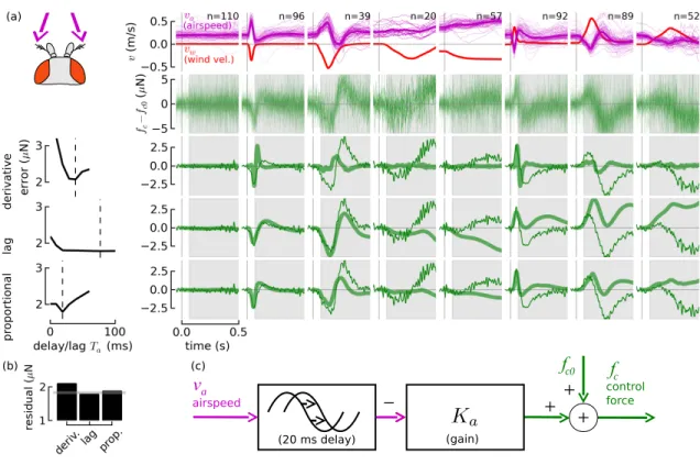
Figure 3.3: System identication supports a proportional controller with a 20 ms delay as the antennae feedback controller. The eect of visual stimuli was eliminated by considering only responses during the early, pre-visual period (unshaded portion of plots). A range of tunnel-frame wind stimuli conditions vw (a) (top row, red) and corresponding y-frame airspeed stimuli va (magenta) were presented to ies. Their force responsesfc, recentered to zero, are shown in the second row. We proposed three controller models, derivative, lag, and proportional, and t them to the ies' input-output behavior. To t the delay or lag time, we performed the t for a range of delays (left column) and chose the delay or lag (dashed vertical line) with the lowest residual error. We simulated each controller with the mean va as input (thick green line, lower three rows) and compared the response to ies' mean force respones (thin green line). The model and the data diverge after 0.1 s because of the eect of the visual response. The residual error for all trajectories and conditions for each controller is shown in (b), compared with the standard deviation for condition 1 (grey line), which had no input. The simplest controller that can explain the observed controller with delay, shown it in block diagram form (c).
The simplest controller that could explain observed behavior with reasonable error was
the proportional controller with a short delay, shown in block diagram form in Figure3.3. The gain for the chosen proportional controller is 7.8×10⁻⁶, similar to damping the damping coecient of the wings at 8 ×10⁻⁶, so the eect of the active antennae response is to essentially double wing damping.
We remark that the model for the airspeed feedback exhibits the behavior observed in the previous chapter, that the feedback response in eect augments the gust. The eect is observed in about equal measure in both directions. The y appears to be regulating around a desired airspeed, decelerating or accelerating if it is not matched. If subject to a headwind gust, a y with intact aristae would be expected to quickly decelerate to match the airspeed, as in shown Figure 2.5.
We emphasize that a derivative controller cannot account for the observed behavior. A derivative controller would exhibit a very weak force response in gentle gusts (as shown in the derivative controller's response to gentle gusts in Figure 3.3) because of the small airspeed derivative, but this is not observed.
3.6 Visual model
Next we found a model for visual feedback by subjecting arista-ablated ies to visual stimuli so that their feedback response was due only to vision. We assumed feedback from the antennae became steady-state after arista removal because of the slow adaptation observed in all mechanosensory systems.
We proposed three simple linear models, proportional, integral, and proportional + inte- gral controllers, with corresponding frequency-domain representationse−sTvKvp,e−sTv1sKvi, e−sTv(1sKvi+Kvp). A derivative model was eliminated out of hand because it would require an extremely long associated delay (taking a derivative adds phase leadthe opposite of a delay). Visual velocity timecourses were chosen by nding ies' mean velocity responses to the wind stimuli chosen in the previous section. The t procedure was performed as described in the previous section, except with visual velocity vv as the input and the fol- lowing changes: (1) Fits were performed over 0.5 s rather than just the 60 ms pre-visual period. Longer t periods did not yield reasonable ts (t gains too small), possibly because of visual motion adaptation in the vision system [75, 76]. (2) We used conditions 2, 3, 5, and 6 (from the left) of Figure 3.4 to perform the t. The other conditions had a much
lower signal-to-noise ratio. (3) Condition 2 was used for nding time delays. For the pro- portional+integral controller, the least-squares was extended to t to t both gains at once, and the median of each gain vector was taken.
The visual feedback model includes avdinput, which was included to be consistent with the nding that ies maintain a steady-state groundspeed independent of airspeed [54], a behavior likely dependent on vision.
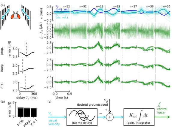
The overall residual error for the three dierent controllers showed comparable perfor- mance (Figure 3.4). The proportional controller was discarded because it could not explain the nding by [54] and reproduced in this lab (data not shown) that ies' groundspeeds are independent of wind velocity, which necessitates a high gain at low frequencies, or a more complicated wind-speed estimator (see Discussion) to eliminate steady-state error. The pro- portional+integral controller was slightly better, but is more complicated. For the sake of simplicity, and because it required a more neurologically plausible shorter delay (60 ms vs 150 ms), we prefer the integral controller.
(60 ms delay) (gain, integrator)
_
visual velocity
vv
fc control force
(b) (c)
prop.integ.P + I
+ + vd desired groundspeed
Figure 3.4: A good t for the visual controller is an integral controller with a 60 ms time delay. The eect of antenna feedback was eliminated by removing the aristae. A range of tunnel-frame visual stimuli conditions vp (a) (top row, dark blue) and corresponding y-frame visual stimuli vv (turquoise) were presented to ies. Their force responses fc, recentered to zero, are shown in the second row. We proposed three controller models, proportional, integral, and proportional+integral, and t them to the ies' input-output behavior. To nd the correct delay, we performed the t for a range of delays (left column) and chose the delay (dashed vertical line) with the lowest residual error. For validation we simulated each controller with the meanvv as input (thick green line, lower three rows) and c