Applied Fluid Mechanics Lab Manual
APPLIED FLUID MECHANICS LAB MANUAL
HABIB AHMARI AND SHAH MD IMRAN KABIR
Mavs Open Press
Arlington
Applied Fluid Mechanics Lab Manual by Habib Ahmari and Shah Md Imran Kabir is licensed under a Creative Commons Attribution 4.0 International License, except where otherwise noted.
CONTENTS
About the Publisher Mavs Open Press
vii
About This Project ix
Acknowledgments xi
LAB MANUAL
Experiment #1: Hydrostatic Pressure 3
Experiment #2: Bernoulli's Theorem Demonstration 13
Experiment #3: Energy Loss in Pipe Fittings 24
Experiment #4: Energy Loss in Pipes 33
Experiment #5: Impact of a Jet 43
Experiment #6: Orifice and Free Jet Flow 50
Experiment #7: Osborne Reynolds' Demonstration 59
Experiment #8: Free and Forced Vortices 66
Experiment #9: Flow Over Weirs 76
Experiment #10: Pumps 84
References 101
Links by Chapter 102
Image Credits 104
ABOUT THE PUBLISHER
MAVS OPEN PRESS
ABOUT MAVS OPEN PRESS
Creation of this resource was supported by Mavs Open Press, operated by the University of Texas at Arlington Libraries (UTA Libraries). Mavs Open Press offers no-cost services for UTA faculty, staff, and students who wish to openly publish their scholarship. The Libraries’ program provides human and technological resources that empower our communities to publish new open access journals, to convert traditional print journals to open access publications, and to create or adapt open educational resources (OER). Resources published by Mavs Open Press are openly licensed using Creative Commons licenses and are offered in various e-book formats free of charge. Optional print copies may be available through the UTA Bookstore or can be purchased through print-on-demand services, such as Lulu.com.
ABOUT OER
OER are free teaching and learning materials that are licensed to allow for revision and reuse. They can be fully self-contained textbooks, videos, quizzes, learning modules, and more. OER are distinct from public resources in that they permit others to use, copy, distribute, modify, or reuse the content.
The legal permission to modify and customize OER to meet the specific learning objectives of a particular course make them a useful pedagogical tool.
ABOUT PRESSBOOKS
Pressbooks is a web-based authoring tool based on WordPress, and it is the primary tool that Mavs Open Press (in addition to many other open textbook publishers) uses to create and adapt open textbooks. In May 2018, Pressbooks announced theirAccessibility Policy, which outlines their efforts and commitment to making their software accessible. Please note that Pressbooks no longer supports use on Internet Explorer as there are important features in Pressbooks that Internet Explorer does not support.
The following browsers are best to use for Pressbooks:
• Firefox
• Chrome
• Safari
• Edge CONTACT US
Information about open education at UTA is available online. If you are an instructor who is using this OER for a course, please let us know by filling out our OER Adoption Form. Contact us at [email protected] for other inquiries related to UTA Libraries publishing services.
ABOUT THIS PROJECT
UTA CARES GRANT PROGRAM
Creation of this OER was funded by the UTA CARES Grant Program, which is sponsored by UTA Libraries. Under the auspices of UTA’s Coalition for Alternative Resources in Education for Students (CARES), the grant program supports educators interested in practicing open education through the adoption of OER and, when no suitable open resource is available, through the creation of new OER or the adoption of library-licensed or other free content. Additionally, the program promotes innovation in teaching and learning through the exploration of open educational practices, such as collaborating with students to produce educational content of value to a wider community.
Information about the grant program and funded projects is available online.
OVERVIEW
This OER is designed for a junior-level lab in applied fluid mechanics (CE 3142) at UTA. The lack of standard material for the fluid mechanics laboratory course causes students to seek help from several textbooks in the subject area for the theoretical background of experiments, which costs them money and time; others seek out online resources for lab demonstrations. Even though free resources (e.g.
lab manuals, videos, lab reports) are increasingly available on the Internet, they are too frequently inadequate and unreliable. This manual supports students by providing streamlined, vetted, and self- paced content, which frees students’ time and saves them money. The OER includes customized lab manuals, educational videos, and an interactive lab report preparation workbooks for ten fluid mechanics experiments. Each section includes theory, practical applications, objectives, experimental procedure, and post-experiment questions. Preparation of result tables and charts are automated within the workbook for each experiment to facilitate answering post-experiment questions and writing lab reports.
CREATION PROCESS
In Summer 2017, Dr. Habib Ahmari taught the Fluid Mechanics Lab at UTA for the first time. He found students struggling with lab manuals that were prepared by previous instructors. Despite the fact that laboratory courses are considered essential components of engineering programs, there are no standard textbooks available for such courses. The lab teaching materials are usually developed by lab instructors (as handouts) or lab equipment manufactures as instruction manuals. These types of course materials are narratives and do not match very well with the nature of these courses;
thus students rarely make connections with them. After teaching the course for two semesters, Dr.
Ahmari realized it was very difficult for students to visualize the experimental procedures by reading these narratives. He also noticed that some students would videotape him or teaching assistants demonstrating the experimental procedure for future references. These observations triggered the idea of developing an OER for the course.
Dr. Ahmari was awarded a UTA CARES Innovation Grant in 2018 to develop an OER to support transitioning the traditional Fluid Mechanics Lab to a media-rich, student-paced learning environment. Shah Md Imran Kabir (graduate student) and Andrew Czubai, Ankur Patel, Nicholas Sopko (undergraduate students) were recruited for this project. This dedicated team worked on this project during the summer to make sure the platform would be ready for implementation for Fall 2018. Creation of the OER project included five steps. The first step was to shoot eleven educational videos of the lab experiments. For this work, two groups of two students were formed. The first group assisted with preparing scripts for videos, demonstrating experiments in the Fluid Mechanics Laboratory of the Civil Engineering Department, and providing voice over of the video. The second group performed video recording, editing, and adding closed captioning. In the next step, lab manuals for ten lab experiments were developed by Dr. Ahmari and his graduate student, Shah Md Imran Kabir. The lab manual was reviewed by a professional editor to enhance the quality of the material.
Next, the team prepared the necessary workbooks for each of the experiments that can be used by students to record their raw data as input. The result tables and graphs will be automatically prepared within the workbook as output. All components of this OER (i.e. lab manuals, videos, and report preparing workbooks) were shared with students enrolled in Fluid Mechanics Lab in Fall 2018 via Blackboard. In Summer 2019, the manual was published in Pressbooks with videos and workbooks embedded in the text.
ABOUT THE AUTHORS
Habib Ahmari, Ph. D., P.E. is an Assistant Professor of Instruction and the Director of the Learning Center in the Department of Civil Engineering at UTA. He has more than 15 years of industry, education, and research experience. He has developed and taught several graduate and undergraduate courses in the area of water resources engineering.
Shah Md Imran Kabir is a graduate student in the Department of Civil Engineering at UTA. He completed his B.Sc. in water resources engineering from Bangladesh University of Engineering and Technology. He has 2 years of working experience in the water resources engineering industry.
ACKNOWLEDGMENTS
LEAD AUTHORS
Habib Ahmari, Ph.D., P.E.– Assistant Professor of Instruction, University of Texas at Arlington Shah Md Imran Kabir – Graduate Teaching Assistant, University of Texas at Arlington
CONTRIBUTORS
Andrew Czubai – University of Texas at Arlington undergraduate student, Civil Engineering Ankur Patel – University of Texas at Arlington undergraduate student, Civil Engineering Nicholas Sopko – University of Texas at Arlington undergraduate student, Civil Engineering EDITOR
Ginny Bowers – former administrative assistant for UTA Department of Civil Engineering (retired) ADDITIONAL THANKS TO
Michelle Reed, Brittany Griffiths, Kartik Mann, and Thomas Perappadan of UTA Libraries for assisting in the publication of this resource.
ABOUT THE COVER
Brittany Griffiths, UTA Libraries’ Publishing Specialist, designed the cover for this OER. The image used isCascade and Ponds, Cooper Street, Arlington, Texas,and was taken by the author, Habib Ahmari.
LAB MANUAL
Basic knowledge about fluid mechanics is required in various areas of water resources engineering such as designing hydraulic structures and turbomachinery. The applied fluid mechanics laboratory course is designed to enhance civil engineering students’ understanding and knowledge of experimental methods and the basic principle of fluid mechanics and apply those concepts in practice.
The lab manual provides students with an overview of ten different fluid mechanics laboratory experiments and their practical applications. The objective, practical applications, methods, theory, and the equipment required to perform each experiment are presented. The experimental procedure, data collection, and presenting the results are explained in detail.
EXPERIMENT #1: HYDROSTATIC PRESSURE
1. INTRODUCTION
Hydrostatic forces are the resultant force caused by the pressure loading of a liquid acting on submerged surfaces. Calculation of the hydrostatic force and the location of the center of pressure are fundamental subjects in fluid mechanics. The center of pressure is a point on the immersed surface at which the resultant hydrostatic pressure force acts.
2. PRACTICAL APPLICATION
The location and magnitude of water pressure force acting on water-control structures, such as dams, levees, and gates, are very important to their structural design. Hydrostatic force and its line of action is also required for the design of many parts of hydraulic equipment.
3. OBJECTIVE
The objectives of this experiment are twofold:
• To determine the hydrostatic force due to water acting on a partially or fully submerged surface;
• To determine, both experimentally and theoretically, the center of pressure.
4. METHOD
In this experiment, the hydrostatic force and center of pressure acting on a vertical surface will be determined by increasing the water depth in the apparatus water tank and by reaching an equilibrium condition between the moments acting on the balance arm of the test apparatus. The forces which create these moments are the weight applied to the balance arm and the hydrostatic force on the vertical surface.
5. EQUIPMENT
Equipment required to carry out this experiment is the following:
• Armfield F1-12 Hydrostatic Pressure Apparatus,
• A jug, and
• Calipers or rulers, for measuring the actual dimensions of the quadrant.
6. EQUIPMENT DESCRIPTION
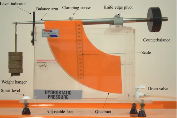
The equipment is comprised of a rectangular transparent water tank, a fabricated quadrant, a balance arm, an adjustable counter-balance weight, and a water-level measuring device (Figure 1.1).
The water tank has a drain valve at one end and three adjustable screwed-in feet on its base for leveling the apparatus. The quadrant is mounted on a balance arm that pivots on knife edges. The knife edges coincide with the center of the arc of the quadrant; therefore, the only hydrostatic force acting on the vertical surface of the quadrant creates moment about the pivot point. This moment can be counterbalanced by adding weight to the weight hanger, which is located at the left end of the balance arm, at a fixed distance from the pivot. Since the line of actions of hydrostatic forces applied on the curved surfaces passes through the pivot point, the forces have no effect on the moment. The hydrostatic force and its line of action (center of pressure) can be determined for different water depths, with the quadrant’s vertical face either partially or fully submerged.
A level indicator attached to the side of the tank shows when the balance arm is horizontal. Water is admitted to the top of the tank by a flexible tube and may be drained through a cock in the side of the tank. The water level is indicated on a scale on the side of the quadrant [1].
Figure 1.1: Armfield F1-12 Hydrostatic Pressure Apparatus
7. THEORY
In this experiment, when the quadrant is immersed by adding water to the tank, the hydrostatic force applied to the vertical surface of the quadrant can be determined by considering the following [1]:
• The hydrostatic force at any point on the curved surfaces is normal to the surface and resolves through the pivot point because it is located at the origin of the radii. Hydrostatic forces on the upper and lower curved surfaces, therefore, have no net effect – no torque to affect the equilibrium of the assembly because the forces pass through the pivot.
• The forces on the sides of the quadrant are horizontal and cancel each other out (equal and opposite).
• The hydrostatic force on the vertical submerged face is counteracted by the balance weight.
The resultant hydrostatic force on the face can, therefore, be calculated from the value of the balance weight and the depth of the water.
• The system is in equilibrium if the moments generated about the pivot points by the hydrostatic force and added weight (=mg) are equal, i.e.:
where:
m : mass on the weight hanger,
L : length of the balance arm (Figure 1.2) F : Hydrostatic force, and
y : distance between the pivot and the center of pressure (Figure 1.2).
Then, calculated hydrostatic force and center of pressure on the vertical face of the quadrant can be compared with the experimental results.
7.1 HYDROSTATIC FORCE
The magnitude of the resultant hydrostatic force (F) applied to an immersed surface is given by:
where:
Pc:pressure at centroid of the immersed surface, A: area of the immersed surface,
yc: centroid of the immersed surface measured from the water surface, : density of fluid, and
g : acceleration due to gravity.
The hydrostatic force acting on the vertical face of the quadrant can be calculated as:
• Partially immersed vertical plane (Figure 1.2a):
• Fully immersed vertical plane (Figure 1.2b):
where:
B : width of the quadrant face,
d : depth of water from the base of the quadrant, and D : height of the quadrant face.
7.2 THEORETICAL DETERMINATION OF CENTER OF PRESSURE The center of pressure is calculated as:
is the 2ndmoment of area of immersed body about an axis in the free surface. By use of the parallel axes theorem:
where is the depth of the centroid of the immersed surface, and is the 2ndmoment of area of immersed body about the centroidal axis. is calculated as:
• Partially immersed vertical plane:
• Fully immersed vertical plane:
The depth of the center of pressure below the pivot point is given by:
in which H is the vertical distance between the pivot and the base of the quadrant.
Substitution of Equation (6a and 6b) and into (4) and then into (7) yields the theoretical results, as follows:
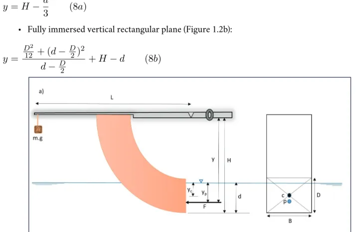
• Partially immersed vertical plane (Figure 1.2a):
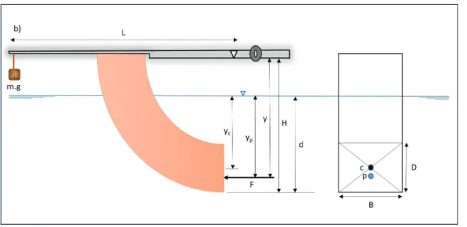
• Fully immersed vertical rectangular plane (Figure 1.2b):
Figure 1.2a: Partially submerged quadrant (c: centroid, p: center of pressure)
Figure 1.2b: Fully submerged quadrant (c: centroid, p: center of pressure)
7.3 EXPERIMENTAL DETERMINATION OF CENTER OF PRESSURE
For equilibrium of the experimental apparatus, moments about the pivot are given by Equation (1).
By substitution of the derived hydrostatic force, F from Equation (3a and b), we have:
• Partially immersed vertical plane (Figure 1.2a):
• Fully immersed vertical rectangular plane (Figure 1.2b):
8. EXPERIMENTAL PROCEDURE
A YouTube element has been excluded from this version of the text. You can view it online here:
https://uta.pressbooks.pub/appliedfluidmechanics/?p=5
A YouTube element has been excluded from this version of the text. You can view it online here:
https://uta.pressbooks.pub/appliedfluidmechanics/?p=5
Begin the experiment by measuring the dimensions of the quadrant vertical endface (BandD) and the distances (HandL), and then perform the experiment by taking the following steps:
• Wipe the quadrant with a wet rag to remove surface tension and prevent air bubbles from forming.
• Place the apparatus on a level surface, and adjust the screwed-in feet until the built-in circular spirit level indicates that the base is horizontal. (The bubble should appear in the center of the spirit level.)
• Position the balance arm on the knife edges and check that the arm swings freely.
• Place the weight hanger on the end of the balance arm and level the arm, using the counter weight, so that the balance arm is horizontal.
• Add 50 grams to the weight hanger.
• Add water to the tank and allow time for the water to settle.
• Close the drain valve at the end of the tank, then slowly add water until the hydrostatic force on the end surface of the quadrant is balanced. This can be judged by aligning the base of the balance arm with the top or bottom of the central marking on the balance rest.
• Record the water height, which displayed on the side of the quadrant in mm. If the quadrant
is partially submerged, record the reading in the partially submerged portion of the Raw Data Table.
• Repeat the steps, adding 50 g weight each time, until the final weight of 500 g is reached. When the quadrant is fully submerged, record the readings in the fully submerged part of the Raw Data Table.
• Repeat the procedure in reverse by progressively removing the weights.
• Release the water valve, remove the weights, and clean up any spilled water.
9. RESULTS AND CALCULATIONS
Please visit this link for accessing the excel workbook for this experiment.
9.1 RESULT
Record the following dimensions:
• Height of quadrant endface, D (m) =
• Width of submerged, B (m)=
• Length of balance arm, L (m)=
• Distance from base of quadrant to pivot, H (m)=
All mass and water depth readings should be recorded in the Raw Data Table:
Raw Data Table
Test No. Mass, m (kg) Depth of Immersion, d (m)
Partially submerged
1 2 3 4 5
Fully Submerged
6 7 8 9 10
9.2 CALCULATIONS
Calculate the following for the partially and fully submerged quadrants, and record them in the Result Table:
• Hydrostatic force (F)
• Theoretical depth of center of pressure below the pivot (y)
• Experimental depth of center of pressure below the pivot (y) Result Table
TestNo. Mass
m(kg) Depth of
immersion d(m) Hydrostatic force
F(N) Theoretical depth of center of
pressure (m) Experimental depth of center of pressure (m)
1 2 3 4 5 6 7 8 9 10
10. REPORT
Use the template provided to prepare your lab report for this experiment. Your report should include the following:
• Table (s) of raw data
• Table (s) of results
• Plots of the following graphs:
◦ Hydrostatic force (y-axis) vs depth of immersion (y-axis),
◦ Theoretical depth of center of pressure (y-axis) vs depth of immersion (x-axis),
◦ Experimental depth of center of pressure (y-axis) vs depth of immersion (x-axis),
◦ Theoretical depth of centre of pressure (y-axis) vs experimental depth of center of pressure (x-axis). Calculate and present value for this graph, and
◦ Mass (y-axis) vs depth of immersion (x-axis) on a log-log scale graph.
• Comment on the variations of hydrostatic force with depth of immersion.
• Comment on the relationship between the depth of the center of pressure and the depth of immersion.
• For both hydrostatic force and theoretical depth of center of pressure plotted vs depth of immersion, comment on what happens when the vertical endface of quadrant becomes fully submerged.
• Comment on and explain the discrepancies between the experimental and theoretical results for the center of pressure.
EXPERIMENT #2: BERNOULLI'S THEOREM DEMONSTRATION
1. INTRODUCTION
Energy presents in the form of pressure, velocity, and elevation in fluids with no energy exchange due to viscous dissipation, heat transfer, or shaft work (pump or some other device). The relationship among these three forms of energy was first stated by Daniel Bernoulli (1700-1782), based upon the conservation of energy principle. Bernoulli’s theorem pertaining to a flow streamline is based on three assumptions: steady flow, incompressible fluid, and no losses from the fluid friction. The validity of Bernoulli’s equation will be examined in this experiment.
2. PRACTICAL APPLICATION
Bernoulli’s theorem provides a mathematical means to understanding the mechanics of fluids. It has many real-world applications, ranging from understanding the aerodynamics of an airplane;
calculating wind load on buildings; designing water supply and sewer networks; measuring flow using devices such as weirs, Parshall flumes, and venturimeters; and estimating seepage through soil, etc.
Although the expression for Bernoulli’s theorem is simple, the principle involved in the equation plays vital roles in the technological advancements designed to improve the quality of human life.
3. OBJECTIVE
The objective of this experiment is to investigate the validity of the Bernoulli equation when it is applied to a steady flow of water through a tapered duct.
4. METHOD
In this experiment, the validity of Bernoulli’s equation will be verified with the use of a tapered duct (venturi system) connected with manometers to measure the pressure head and total head at known points along the flow.
5. EQUIPMENT
The following equipment is required to complete the demonstration of the Bernoulli equation experiment:
• F1-10 hydraulics bench,
• F1-15 Bernoulli’s apparatus test equipment, and
• A stopwatch for timing the flow measurement.
6. EQUIPMENT DESCRIPTION
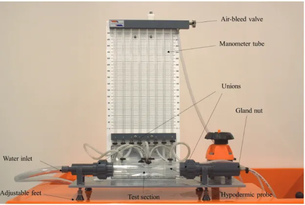
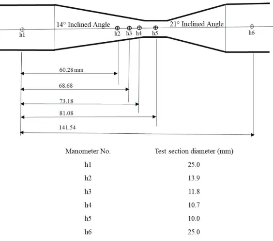
The Bernoulli test apparatus consists of a tapered duct (venturi), a series of manometers tapped into the venturi to measure the pressure head, and a hypodermic probe that can be traversed along the center of the test section to measure the total head. The test section is a circular duct of varying diameter with a 14° inclined angle on one side and a 21° inclined angle on other side. Series of side hole pressure tappings are provided to connect manometers to the test section (Figure 2.1).
Figure 2.1: Armfield F1-15 Bernoulli’s apparatus test equipment
Manometers allow the simultaneous measurement of the pressure heads at all of the six sections along the duct. The dimensions of the test section, the tapping positions, and the test section diameters are shown in Figure 2.2. The test section incorporates two unions, one at either end, to facilitate reversal for convergent or divergent testing. A probe is provided to measure the total pressure head along the test section by positioning it at any section of the duct. This probe may be moved after slackening the gland nut, which should be re-tightened by hand. To prevent damage, the probe should be fully inserted during transport/storage. The pressure tappings are connected to manometers that are mounted on a baseboard. The flow through the test section can be adjusted by the apparatus control valve or the bench control valve [2].
Figure 2.2: Test sections, manometer positions, and diameters of the duct along the test section
7. THEORY
Bernoulli’s theorem assumes that the flow is frictionless, steady, and incompressible. These assumptions are also based on the laws of conservation of mass and energy. Thus, the input mass and energy for a given control volume are equal to the output mass and energy:
These two laws and the definition of work and pressure are the basis for Bernoulli’s theorem and can be expressed as follows for any two points located on the same streamline in the flow:
where:
P: pressure,
g: acceleration due to gravity, v: fluid velocity, and
z: vertical elevation of the fluid.
In this experiment, since the duct is horizontal, the difference in height can be disregarded, i.e., z1=z2 The hydrostatic pressure (P) along the flow is measured by manometers tapped into the duct. The pressure head (h), thus, is calculated as:
Therefore, Bernoulli’s equation for the test section can be written as:
in which is called the velocity head (hd).
The total head (ht) may be measured by the traversing hypodermic probe. This probe is inserted into the duct with its end-hole facing the flow so that the flow becomes stagnant locally at this end; thus:
The conservation of energy or the Bernoulli’s equation can be expressed as:
The flow velocity is measured by collecting a volume of the fluid (V) over a time period (t). The flow rate is calculated as:
The velocity of flow at any section of the duct with a cross-sectional area of is determined as:
For an incompressible fluid, conservation of mass through the test section should be also satisfied (Equation 1a), i.e.:
8. EXPERIMENTAL PROCEDURE
A YouTube element has been excluded from this version of the text. You can view it online here:
https://uta.pressbooks.pub/appliedfluidmechanics/?p=50
• Place the apparatus on the hydraulics bench, and ensure that the outflow tube is positioned above the volumetric tank to facilitate timed volume collections.
• Level the apparatus base by adjusting its feet. (A sprit level is attached to the base for this purpose.) For accurate height measurement from the manometers, the apparatus must be horizontal.
• Install the test section with the 14° tapered section converging in the flow direction. If the test section needs to be reversed, the total head probe must be retracted before releasing the mounting couplings.
• Connect the apparatus inlet to the bench flow supply, close the bench valve and the apparatus flow control valve, and start the pump. Gradually open the bench valve to fill the test section with water.
• The following steps should be taken to purge air from the pressure tapping points and manometers:
◦ Close both the bench valve and the apparatus flow control valve.
◦ Remove the cap from the air valve, connect a small tube from the air valve to the
volumetric tank, and open the air bleed screw.
◦ Open the bench valve and allow flow through the manometers to purge all air from them, then tighten the air bleed screw and partly open the bench valve and the apparatus flow control valve.
◦ Open the air bleed screw slightly to allow air to enter the top of the manometers (you may need to adjust both valves to achieve this), and re-tighten the screw when the manometer levels reach a convenient height. The maximum flow will be determined by having a maximum (h1) and minimum (h5) manometer readings on the baseboard.
If needed, the manometer levels can be adjusted by using an air pump to pressurize them. This can be accomplished by attaching the hand pump tube to the air bleed valve, opening the screw, and pumping air into the manometers. Close the screw, after pumping, to retain the pressure in the system.
• Take readings of manometersh1to h6when the water level in the manometers is steady. The total pressure probe should be retracted from the test section during this reading.
• Measure the total head by traversing the total pressure probe along the test section from h1to h6.
• Measure the flow rate by a timed volume collection. To do that, close the ball valve and use a stopwatch to measure the time it takes to accumulate a known volume of fluid in the tank, which is read from the sight glass. You should collect fluid for at leastone minuteto minimize timing errors. You may repeat the flow measurement twice to check for repeatability. Be sure that the total pressure probe is retracted from the test section during this measurement.
• Reduce the flow rate to give the head difference of about 50 mm between manometers 1 and 5 (h1-h5). This is the minimum flow experiment. Measure the pressure head, total head, and flow.
• Repeat the process for one more flow rate, with the (h1-h5) difference approximately halfway between those obtained for the minimum and maximum flows. This is the average flow experiment.
• Reverse the test section (with the21° tapered sectionconverging in the flow direction) in order to observe the effects of a more rapidly converging section. Ensure that the total pressure probe is fully withdrawn from the test section, but not pulled out of its guide in the downstream coupling. Unscrew the two couplings, remove the test section and reverse it, then re-assemble it by tightening the couplings.
• Perform three sets of flow, and conduct pressure and flow measurements as above.
9. RESULTS AND CALCULATIONS
Please visit this link for accessing excel workbook for this experiment.
9.1. RESULTS
Enter the test results into the Raw Data Tables.
Raw Data Table
Position 1: Tapering 14° to 21°
Test Section Volume (Litre) Time (sec) Pressure Head (mm) Total Head (mm) h1
h2
h3
h4
h5
h6
h1
h2
h3
h4
h5
h6
h1
h2
h3
h4
h5
h6
Raw Data Table
Position 2: Tapering 21° to 14°
Test Section Volume (Litre) Time (sec) Pressure Head (mm) Total Head (mm) h1
h2
h3
h4
h5
h6
h1
h2
h3
h4
h5
h6
h1
h2
h3
h4
h5
h6
9.2 CALCULATIONS
For each set of measurements, calculate the flow rate; flow velocity, velocity head, and total head, (pressure head+ velocity head). Record your calculations in the Result Table.
Result Table
Position 1: Tapering 14° to 21°
TestNo. Test Section Distance into duct
(m)
Area (m²)Flow Flow Rate
(m³/s) Velocity
(m/s) Pressure
Head (m) Velocity Head (m)
Calculated Total Head (m)
Measured Total Head (m)
1
h1 0 0.00049
h2 0.06028 0.00015
h3 0.06868 0.00011
h4 0.07318 0.00009
h5 0.08108 0.000079
h6 0.14154 0.00049
2
h1 0 0.00049
h2 0.06028 0.00015
h3 0.06868 0.00011
h4 0.07318 0.00009
h5 0.08108 0.000079
h6 0.14154 0.00049
3
h1 0 0.00049
h2 0.06028 0.00015
h3 0.06868 0.00011
h4 0.07318 0.00009
h5 0.08108 0.000079
h6 0.14154 0.00049
Position 2: Tapering 21° to 14°
TestNo. Test Section Distance into duct
(m)
Area (m²)Flow Flow Rate
(m³/s) Velocity
(m/s) Pressure
Head (m) Velocity Head (m)
Calculated Total Head (m)
Measured Total Head (m)
1
h1 0 0.00049
h2 0.06028 0.00015
h3 0.06868 0.00011
h4 0.07318 0.00009
h5 0.08108 0.000079
h6 0.14154 0.00049
2
h1 0 0.00049
h2 0.06028 0.00015
h3 0.06868 0.00011
h4 0.07318 0.00009
h5 0.08108 0.000079
h6 0.14154 0.00049
3
h1 0 0.00049
h2 0.06028 0.00015
h3 0.06868 0.00011
h4 0.07318 0.00009
h5 0.08108 0.000079
h6 0.14154 0.00049
10. REPORT
Use the template provided to prepare your lab report for this experiment. Your report should include the following:
• Table(s) of raw data
• Table(s) of results
• For each test, plot the total head (calculated and measured), pressure head, and velocity head (y-axis) vs. distance into duct (x-axis) from manometer 1 to 6, a total of six graphs. Connect the data points to observe the trend in each graph. Note that the flow direction in duct Position 1 is from manometer 1 to 6; in Position 2, it is from manometer 6 to 1.
• Comment on the validity of Bernoulli’s equation when the flow converges and diverges along the duct.
• Comment on the comparison of the calculated and measured total heads in this experiment.
• Discuss your results, referring, in particular, to the following:
◦ energy loss and how it is shown by the results of this experiment, and
◦ the components of Bernoulli’s equation ( ) and how they vary along the length of the test section. Indicate the points of maximum velocity and minimum pressure.
EXPERIMENT #3: ENERGY LOSS IN PIPE FITTINGS
1. INTRODUCTION
Two types of energy loss predominate in fluid flow through a pipe network; major losses, and minor losses. Major losses are associated with frictional energy loss that is caused by the viscous effects of the medium and roughness of the pipe wall. Minor losses, on the other hand, are due to pipe fittings, changes in the flow direction, and changes in the flow area. Due to the complexity of the piping system and the number of fittings that are used, the head loss coefficient (K) is empirically derived as a quick means of calculating the minor head losses.
2. PRACTICAL APPLICATION
The term “minor losses”, used in many textbooks for head loss across fittings, can be misleading since these losses can be a large fraction of the total loss in a pipe system. In fact, in a pipe system with many fittings and valves, the minor losses can be greater than the major (friction) losses. Thus, an accurate K value for all fittings and valves in a pipe system is necessary to predict the actual head loss across the pipe system. K values assist engineers in totaling all of the minor losses by multiplying the sum of the K values by the velocity head to quickly determine the total head loss due to all fittings. Knowing the K value for each fitting enables engineers to use the proper fitting when designing an efficient piping system that can minimize the head loss and maximize the flow rate.
3. OBJECTIVE
The objective of this experiment is to determine the loss coefficient (K) for a range of pipe fittings, including several bends, a contraction, an enlargement, and a gate valve.
4. METHOD
The head loss coefficients are determined by measuring the pressure head differences across a number of fittings that are connected in series, over a range of steady flows, and applying the energy equation between the sections before and after each fitting.
5. EQUIPMENT
The following equipment is required to perform the energy loss in pipe fittings experiment:
• F1-10 hydraulics bench,
• F1-22 Energy losses in bends apparatus,
• Stopwatch for timing the flow measurement,
• Clamps for pressure tapping connection tubes,
• Spirit level, and
• Thermometer.
6. EQUIPMENT DESCRIPTION
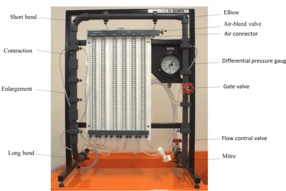
The energy loss in fittings apparatus consists of a series of fittings, a flow control valve, twelve manometers, a differential pressure gauge, and an air-bleed valve (Figure 3.1).
The fittings listed below, connected in a series configuration, will be examined for their head loss coefficient (K):
• long bend,
• area enlargement,
• area contraction,
• elbow,
• short bend,
• gate valve, and
• mitre.
Figure 3.1: F1-22 Energy Losses in Pipe Fittings Apparatus
The manometers are tapped into the pipe system (one before and one after each fitting, except for the
gate valve) to measure the pressure head difference caused by each fitting. The pressure difference for the valve is directly measured by the differential pressure gauge. The air-bleed valve facilitates purging the system and adjusting the water level in the manometers to a convenient level, by allowing air to enter them. Two clamps, which close off the tappings to the mitre, are introduced while experiments are being performed on the gate valve. The flow rate is controlled by the flow control valve [3].
The internal diameter of the pipe and all fittings, except for the enlargement and contraction, is 0.0183 m. The internal diameter of the pipe at the enlargement’s outlet and the contraction’s inlet is 0.0240 m.
7. THEORY
Bernoulli’s equation can be used to evaluate the energy loss in a pipe system:
In this equation , , and z are pressure head, velocity head, and potential head, respectively. The total head loss, hL, includes both major and minor losses.
If the diameter through the pipe fitting is kept constant, then . Therefore, if the change in elevation head is neglected, the manometric head difference is the static head difference that is equal to the minor loss through the fitting.
in which and are manometer readings before and after the fitting.
The energy loss that occurs in a pipe fitting can also be expressed as a fraction (K ) of the velocity head through the fitting:
where:
K: loss coefficient, and
v: mean flow velocity into the fitting.
Because of the complexity of the flow in many fittings, K is usually determined by experiment [3]. The head loss coefficient (K) is calculated as the ratio of the manometric head difference between the input and output of the fitting to the velocity head.
Due to the change in the pipe cross-sectional area in enlargement and contraction fittings, the velocity difference cannot be neglected. Thus:
Therefore, these types of fittings experience an additional change in static pressure, i.e.:
.
This value will be negative for the contraction since and it will be positive for enlargement because . From Equation (5), note that will be negative for the enlargement.
The pressure difference ( ) between before and after the gate valve is measured directly using the pressure gauge. This can then be converted to an equivalent head loss by using the conversion ratio:
1 bar= 10.2 m water
The loss coefficient for the gate valve may then be calculated by using Equation (4).
To identify the flow regime through the fitting, the Reynolds number is calculated as:
where v is the cross-sectional mean velocity, D is the pipe diameter and is the fluid kinematic viscosity (Figure 3.2).
Figure 3.2: Kinematic Viscosity of Water (v) at Atmospheric Pressure
8. EXPERIMENTAL PROCEDURE
A YouTube element has been excluded from this version of the text. You can view it online here:
https://uta.pressbooks.pub/appliedfluidmechanics/?p=127
It is not possible to measure head due to all of the fittings simultaneously; therefore, it is necessary to run two separate experiments.
PART A:
In this part, head losses caused by fittings, except for the gate valve, will be measured; therefore, this valve should be kept fully open throughout Part A. The following steps should be followed for this part:
• Set up the apparatus on the hydraulics bench and ensure that its base is horizontal.
• Connect the apparatus inlet to the bench flow supply, run the outlet extension tube to the volumetric tank, and secure it in place.
• Open the bench valve, the gate valve, and the flow control valve, and start the pump to fill the pipe system and manometers with water. Ensure that the air-bleed valve is closed.
• To purge air from the pipe system and manometers, connect a bore tubing from the air valve to the volumetric tank, remove the cap from the air valve, and open the air-bleed screw to allow flow through the manometers. Tighten the air-bleed screw when no air bubbles are observed in the manometers.
• Set the flow rate at approximately 17 liters/minute. This can be achieved by several trials of timed volumetric flow measurements. For flow measurement, close the ball valve, and use a stopwatch to measure the time that it takes to accumulate a known volume of fluid in the tank, which is read from the hydraulics bench sight glass. Collect water for at least one minute to minimize errors in the flow measurement.
• Open the air-bleed screw slightly to allow air to enter the top of the manometers; re-tighten the screw when the manometer levels reach a convenient height. All of the manometer levels should be on scale at the maximum flow rate. These levels can be adjusted further by using the air-bleed screw and the hand pump. The air-bleed screw controls the air flow through the air valve, so when using the hand pump, the bleed screw must be open. To retain the hand pump pressure in the system, the screw must be closed after pumping [3].
• Take height readings from all manometers after the levels are steady.
• Repeat this procedure to give a total of at least five sets of measurements over a flow range of 8 – 17 liters per minute.
• Measure the outflow water temperature at the lowest flow rate. This, together with Figure 3.2, is used to determine the Reynolds number.
PART B:
In this experiment, the head loss across the gate valve will be measured by taking the following steps:
• Clamp off the connecting tubes to the mitre bend pressure tappings to prevent air being drawn into the system.
• Open the bench valve and set the flow at the maximum flow in Part A (i.e., 17 liter/min); fully open the gate valve and flow control valve.
• Adjust the gate valve until 0.3 bar of head difference is achieved.
• Determine the volumetric flow rate.
• Repeat the experiment for 0.6 and 0.9 bars of pressure difference.
9. RESULTS AND CALCULATIONS
Please visit this link for accessing excel workbook for this experiment.
9.1. RESULTS
Record all of the manometer and pressure gauge readings, as well as the volumetric measurements, in the Raw Data Tables.
Raw Data Tables
Part A – Head Loss Across Pipe Fittings
Test No. 1: Volume Collected (liters): Time (s):
Fitting h1(m) h2(m)
Enlargement Contraction Long Bend Short Bend Elbow Mitre
Test No. 2: Volume Collected (liters): Time (s):
Enlargement Contraction Long Bend Short Bend Elbow Mitre
Test No. 3: Volume Collected (liters): Time (s):
Enlargement Contraction Long Bend Short Bend Elbow Mitre
Test No. 4: Volume Collected (liters): Time (s):
Enlargement Contraction Long Bend Short Bend Elbow Mitre
Test No. 5: Volume Collected (liters): Time (s):
Enlargement Contraction Long Bend Short Bend Elbow Mitre
Part B – Head Loss Across Gate Valve
Head Loss (bar) Volume (liters) Time (s)
0.3 0.6 0.9 Water Temperature:
9.2. CALCULATIONS
Calculate the values of the discharge, flow velocity, velocity head, and Reynolds number for each experiment, as well as the K values for each fitting and the gate valve. Record your calculations in the following sample Result Tables.
Result Table
Part A – Head Loss Across Pipe Fittings
Test No: Flow Rate Q (m3/s): Velocity v (m/s):
Fitting h1(m) h2(m) =h1– h2(m) Corrected (m) v2/2g
(m) K Reynolds
Number Enlargement
Contraction Long Bend Short Bend
Elbow Mitre
Part B – Head Loss Across Pipe Fittings
Head Loss Volume
(m3) Time (s) Flow Rate Q
(m3/s) Velocity
(m/s) v2/2g (m) K Reynolds
Number
(bar) (m)
0.3 0.6 0.9
10. REPORT
Use the template provided to prepare your lab report for this experiment. Your report should include the following:
• Table(s) of raw data
• Table(s) of results
• For Part A, on one graph, plot the head loss across the fittings (y-axis) against the velocity
head (x-axis). On the second graph, plot the K values for the fittings (y-axis) against the flow rate Q (x-axis).
• For Part B, on one graph, plot the valve head losses (y-axis) against the velocity head (x- axis). On the second graph, plot the K values for the valve (y-axis) against the flow rate Q (x- axis).
• Comment on any relationships noticed in the graphs for Parts A and B. What is the dependence of head losses across pipe fittings upon the velocity head?
• Is it justifiable to treat the loss coefficient as constant for a given fitting?
• In Part B, how does the loss coefficient for a gate valve vary with the extent of opening the valve?
• Examine the Reynolds number obtained. Are the flows laminar or turbulent?
EXPERIMENT #4: ENERGY LOSS IN PIPES
1. INTRODUCTION
The total energy loss in a pipe system is the sum of the major and minor losses. Major losses are associated with frictional energy loss that is caused by the viscous effects of the fluid and roughness of the pipe wall. Major losses create a pressure drop along the pipe since the pressure must work to overcome the frictional resistance. The Darcy-Weisbach equation is the most widely accepted formula for determining the energy loss in pipe flow. In this equation, the friction factor (f), a dimensionless quantity, is used to describe the friction loss in a pipe. In laminar flows,f is only a function of the Reynolds number and is independent of the surface roughness of the pipe. In fully turbulent flows, f depends on both the Reynolds number and relative roughness of the pipe wall. In engineering problems, f is determined by using the Moody diagram.
2. PRACTICAL APPLICATION
In engineering applications, it is important to increase pipe productivity, i.e. maximizing the flow rate capacity and minimizing head loss per unit length. According to the Darcy-Weisbach equation, for a given flow rate, the head loss decreases with the inverse fifth power of the pipe diameter. Doubling the diameter of a pipe results in the head loss decreasing by a factor of 32 (≈97% reduction), while the amount of material required per unit length of the pipe and its installation cost nearly doubles. This means that energy consumption, to overcome the frictional resistance in a pipe conveying a certain flow rate, can be significantly reduced at a relatively small capital cost.
3. OBJECTIVE
The objective of this experiment is to investigate head loss due to friction in a pipe, and to determine the associated friction factor under a range of flow rates and flow regimes, i.e., laminar, transitional, and turbulent.
4. METHOD
The friction factor is determined by measuring the pressure head difference between two fixed points in a straight pipe with a circular cross section for steady flows.
5. EQUIPMENT
The following equipment is required to perform the energy loss in pipes experiment:
• F1-10 hydraulics bench,
• F1-18 pipe friction apparatus,
• Stopwatch for timing the flow measurement,
• Measuring cylinder for measuring very low flow rates,
• Spirit level, and
• Thermometer.
6. EQUIPMENT DESCRIPTION
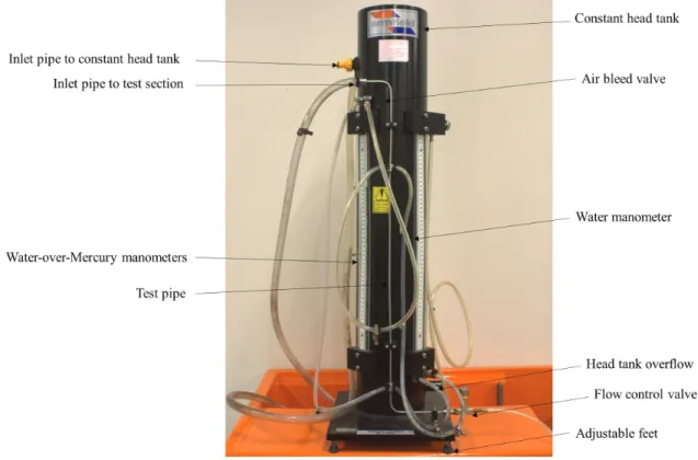
The pipe friction apparatus consists of a test pipe (mounted vertically on the rig), a constant head tank, a flow control valve, an air-bleed valve, and two sets of manometers to measure the head losses in the pipe (Figure 4.1). A set of two water-over-mercury manometers is used to measure large pressure differentials, and two water manometers are used to measure small pressure differentials. When not in use, the manometers may be isolated, using Hoffman clamps.
Since mercury is considered a hazardous substance, it cannot be used in undergraduate fluid mechanics labs. Therefore, for this experiment, the water-over-mercury manometers are replaced with a differential pressure gauge to directly measure large pressure differentials.
This experiment is performed under two flow conditions: high flow rates and low flow rates. For high flow rate experiments, the inlet pipe is connected directly to the bench water supply. For low flow rate experiments, the inlet to the constant head tank is connected to the bench supply, and the outlet at the base of the head tank is connected to the top of the test pipe [4].
The apparatus’ flow control valve is used to regulate flow through the test pipe. This valve should face the volumetric tank, and a short length of flexible tube should be attached to it, to prevent splashing.
The air-bleed valve facilitates purging the system and adjusting the water level in the water manometers to a convenient level, by allowing air to enter them.
Figure 4.1: F1-18 Pipe Friction Test Apparatus
7. THEORY
The energy loss in a pipe can be determined by applying the energy equation to a section of a straight pipe with a uniform cross section:
If the pipe is horizontal:
Sincevin= vout :
The pressure difference (Pout-Pin) between two points in the pipe is due to the frictional resistance, and the head losshLis directly proportional to the pressure difference.
The head loss due to friction can be calculated from the Darcy-Weisbach equation:
where:
: head loss due to flow resistance f: Darcy-Weisbach coefficient
L:pipe length D: pipe diameter v: average velocity
g:gravitational acceleration.
For laminar flow, the Darcy-Weisbach coefficient (or friction factor f ) is only a function of the Reynolds number (Re) and is independent of the surface roughness of the pipe, i.e.:
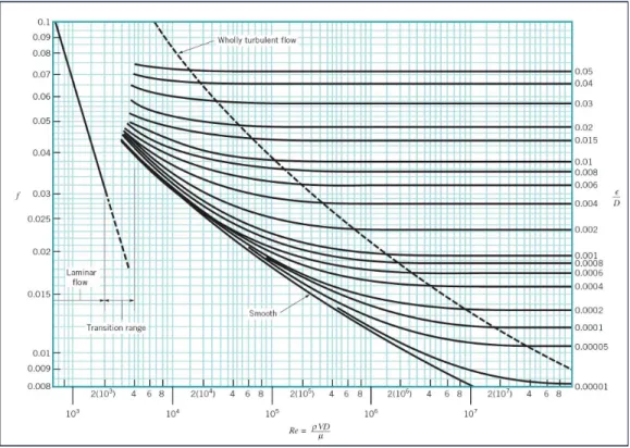
For turbulent flow, f is a function of both the Reynolds number and the pipe roughness height, . Other factors, such as roughness spacing and shape, may also affect the value of f; however, these effects are not well understood and may be negligible in many cases. Therefore,f must be determined experimentally. The Moody diagram relatesfto the pipe wall relative roughness ( /D) and the Reynolds number (Figure 4.2).
Instead of using the Moody diagram, f can be determined by utilizing empirical formulas. These formulas are used in engineering applications when computer programs or spreadsheet calculation methods are employed. For turbulent flow in a smooth pipe, a well-known curve fit to the Moody diagram is given by:
Reynolds number is given by:
where v is the average velocity, D is the pipe diameter, and and are dynamic and kinematic viscosities of the fluid, respectively. (Figure 4.3).
In this experiment, hL is measured directly by the water manometers and the differential pressure gauge that are connected by pressure tappings to the test pipe. The average velocity,v, is calculated from the volumetric flow rate (Q ) as:
The following dimensions from the test pipe may be used in the appropriate calculations [4]:
Length of test pipe = 0.50 m, Diameter of test pipe = 0.003 m.
Figure 4.2: Moody Diagram
Figure 4.3: Kinematic Viscosity of Water (v) at Atmospheric Pressure
8. EXPERIMENTAL PROCEDURE
An interactive or media element has been excluded from this version of the text. You can view it online here: https://uta.pressbooks.pub/appliedfluidmechanics/?p=129
The experiment will be performed in two parts: high flow rates and low flow rates. Set up the equipment as follows:
• Mount the test rig on the hydraulics bench, and adjust the feet with a spirit level to ensure that the baseplate is horizontal and the manometers are vertical.
• Attach Hoffman clamps to the water manometers and pressure gauge connecting tubes, and close them off.
High Flow Rate Experiment
The high flow rate will be supplied to the test section by connecting the equipment inlet pipe to the hydraulics bench, with the pump turned off. The following steps should be followed.
• Close the bench valve, open the apparatus flow control valve fully, and start the pump. Open the bench valve progressively, and run the flow until all air is purged.
• Remove the clamps from the differential pressure gauge connection tubes, and purge any air from the air-bleed valve located on the side of the pressure gauge.
• Close off the air-bleed valve once no air bubbles observed in the connection tubes.
• Close the apparatus flow control valve and take a zero-flow reading from the pressure gauge.
• With the flow control valve fully open, measure the head loss shown by the pressure gauge.
• Determine the flow rate by timed collection.
• Adjust the flow control valve in a step-wise fashion to observe the pressure differences at 0.05 bar increments. Obtain data for ten flow rates. For each step, determine the flow rate by timed collection.
• Close the flow control valve, and turn off the pump.
The pressure difference measured by the differential pressure gauge can be converted to an equivalent head loss (hL) by using the conversion ratio:
1 bar = 10.2 m water Low Flow Rate Experiment
The low flow rate will be supplied to the test section by connecting the hydraulics bench outlet pipe to the head tank with the pump turned off. Take the following steps.
• Attach a clamp to each of the differential pressure gauge connectors and close them off.
• Disconnect the test pipe’s supply tube and hold it high to keep it filled with water.
• Connect the bench supply tube to the head tank inflow, run the pump, and open the bench valve to allow flow. When outflow occurs from the head tank snap connector, attach the test section supply tube to it, ensuring that no air is entrapped.
• When outflow occurs from the head tank overflow, fully open the control valve.
• Remove the clamps from the water manometers’ tubes and close the control valve.
• Connect a length of small bore tubing from the air valve to the volumetric tank, open the air bleed screw, and allow flow through the manometers to purge all of the air from them. Then tighten the air bleed screw.
• Fully open the control valve and slowly open the air bleed valve, allowing air to enter until the manometer levels reach a convenient height (in the middle of the manometers), then close the air vent. If required, further control of the levels can be achieved by using a hand pump to raise the manometer air pressure.
• With the flow control valve fully open, measure the head loss shown by the manometers.
• Determine the flow rate by timed collection.
• Obtain data for at least eight flow rates, the lowest to give hL= 30 mm.
• Measure the water temperature, using a thermometer.
9. RESULTS AND CALCULATIONS
Please use this link for accessing excel workbook for this experiment.
9.1. RESULTS
Record all of the manometer and pressure gauge readings, water temperature, and volumetric measurements, in the Raw Data Tables.
Raw Data Tables: High Flow Rate Experiment
Test No. Head Loss (bar) Volume (Liters) Time (s)
1 2 3 4 5 6 7 8 9 10
Raw Data Tables: Low Flow Rate Experiment
Test No. h1(m) h2(m) Head loss hL(m) Volume (liters) Time (s)
1 2 3 4 5 6 7 8
Water Temperature:
9.2. CALCULATIONS
Calculate the values of the discharge; average flow velocity; and experimental friction factor,fusing Equation 3, and the Reynolds number for each experiment. Also, calculate the theoretical friction factor,f, using Equation 4 for laminar flow and Equation 5 for turbulent flow for a range of Reynolds numbers. Record your calculations in the following sample Result Tables.
Result Table- Experimental Values Test No. Head loss hL
(m) Volume
(liters) Time (s) Discharge
(m3/s) Velocity (m/s) Friction
Factor, f Reynolds Number 1
2 3 4 5 6 7 8 9 10 11 12 13 14 15 16 17 18
Result Table- Theoretical Values
No. Flow Regime Reynolds Number Friction Factor, f
1
Laminar (Equation 4)
100
2 200
3 400
4 800
5 1600
6 2000
7
Turbulent (Equation 5)
4000
8 6000
9 8000
10 10000
11 12000
12 16000
13 20000
10. REPORT
Use the template provided to prepare your lab report for this experiment. Your report should include the following:
• Table(s) of raw data
• Table(s) of results
• Graph(s)
◦ On one graph, plot the experimental and theoretical values of the friction factor, f (y- axis) against the Reynolds number, Re (x-axis) on a log-log scale. The experimental results should be divided into three groups (laminar, transitional, and turbulent) and plotted separately. The theoretical values should be divided into two groups (laminar and turbulent) and also plotted separately.
◦ On one graph, plothL(y-axis) vs. average flow velocity,v(x-axis) on a log-log scale.
• Discuss the following:
◦ Identify laminar and turbulent flow regimes in your experiment. What is the critical Reynolds number in this experiment (i.e., the transitional Reynolds number from laminar flow to turbulent flow)?
◦ Assuming a relationship of the form , calculate K and n values from the graph of experimental data you have plotted, and compare them with the accepted values shown in the Theory section (Equations 4 and 5). What is the cumulative effect of the experimental errors on the values of K and n?
◦ What is the dependence of head loss upon velocity (or flow rate) in the laminar and turbulent regions of flow?
◦ What is the significance of changes in temperature to the head loss?
◦ Compare your results for f with the Moody diagram (Figure 4.2). Note that the pipe utilized in this experiment is a smooth pipe. Indicate any reason for lack of agreement.
◦ What natural processes would affect pipe roughness?
EXPERIMENT #5: IMPACT OF A JET
1. INTRODUCTION
Moving fluid, in natural or artificial systems, may exert forces on objects in contact with it. To analyze fluid motion, a finite region of the fluid (control volume) is usually selected, and the gross effects of the flow, such as its force or torque on an object, is determined by calculating the net mass rate that flows into and out of the control volume. These forces can be determined, as in solid mechanics, by the use of Newton’s second law, or by the momentum equation. The force exerted by a jet of fluid on a flat or curve surface can be resolved by applying the momentum equation. The study of these forces is essential to the study of fluid mechanics and hydraulic machinery.
2. PRACTICAL APPLICATION
Engineers and designers use the momentum equation to accurately calculate the force that moving fluid may exert on a solid body. For example, in hydropower plants, turbines are utilized to generate electricity. Turbines rotate due to force exerted by one or more water jets that are directed tangentially onto the turbine’s vanes or buckets. The impact of the water on the vanes generates a torque on the wheel, causing it to rotate and to generate electricity.
3. OBJECTIVE
The objective of this experiment is to investigate the reaction forces produced by the change in momentum of a fluid flow when a jet of water strikes a flat plate or a curved surface, and to compare the results from this experiment with the computed forces by applying the momentum equation.
4. METHOD
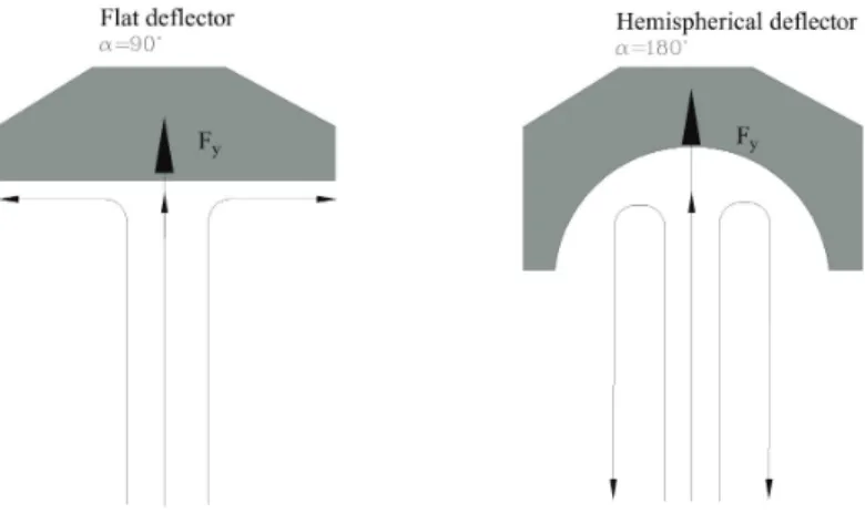
The momentum force is determined by measuring the forces produced by a jet of water impinging on solid flat and curved surfaces, which deflect the jet at different angles.
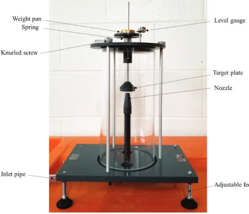
5. EQUIPMENT
The following equipment is required to perform the impact of the jet experiment:
• F1-10 hydraulics bench,
• F1-16 impacts of a jet apparatus with three flow deflectors with deflection angles of 90, 120, and 180 degrees, and