You are introduced to linear least squares regression methods and some of the more common nonlinear models. Principal component analysis is introduced as an aid in characterizing the correlational structure of the data.
REVIEW OF SIMPLE REGRESSION
The Linear Model and Assumptions
The simplest linear model includes only one independent variable and states that the true mean of the dependent variable changes at a constant rate. The observations on the dependent variable Yia are assumed to be random observations from populations of random variables with the mean of each.
Least Squares Estimation
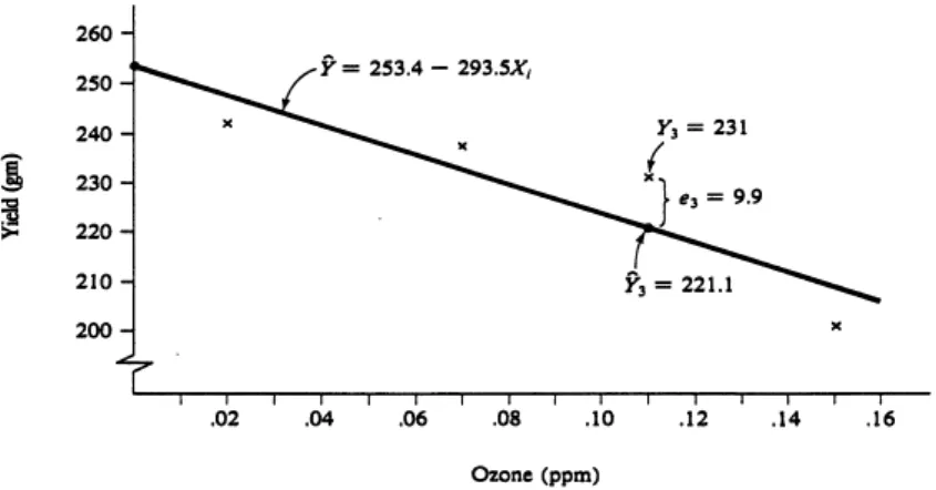
The ozone dose is the average concentration (parts per million, ppm) during the growing season. The least squares regression equation characterizing the effects of ozone on average soybean yield in this study, assuming the linear model is correct, is.
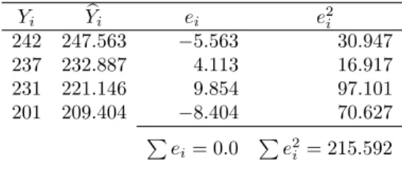
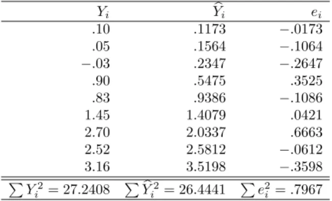
Predicted Values and Residuals
This is a 30 gram decrease in yield over a 0.1 ppm increase in ozone, or a rate of change of -300 grams in Y for each unit increase in X. The pattern of deviations from the regression line, however, suggests that the linear model may not adequately represent the relationship.
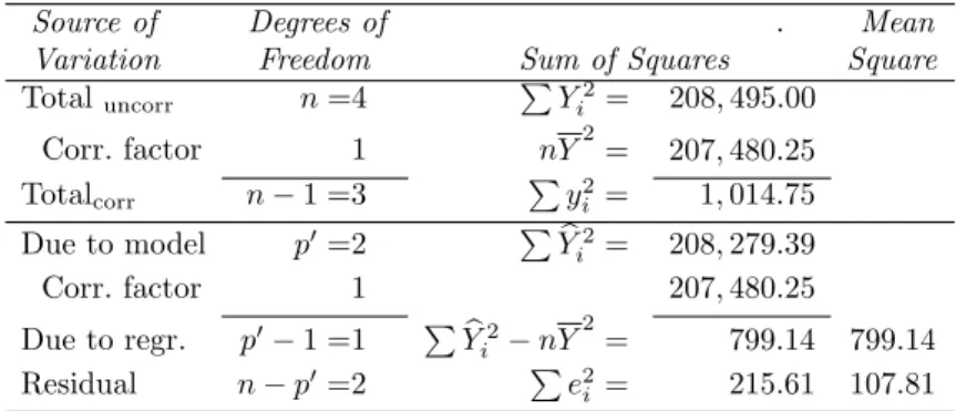
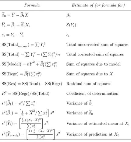
Analysis of Variation in the Dependent Variable
Hereafter, SS(Total) is used to denote the corrected sum of squares of the dependent variable. This is the proportion of the (corrected) sum of squares of Y that can be attributed to the information obtained from the independent variable(s).
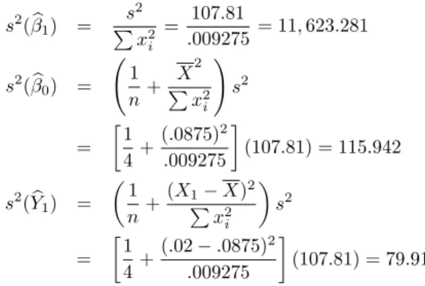
Precision of Estimates
Note that products of the corresponding coefficients are used, while the squares of the coefficients were used in obtaining the variance of a linear function. The variance for the prediction must take into account the fact that the predicted quantity itself is a random variable.
Tests of Significance and Confidence Intervals
The critical value of Student's for the two-tailed alternative hypothesis places probability α/2 in each tail of the distribution. The F-ratio with 1 degree of freedom in the numerator is the square of the corresponding t-statistic.

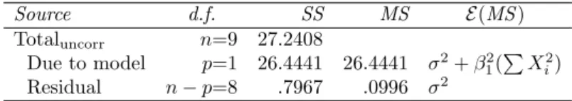
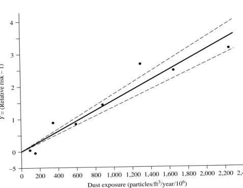
Regression Through the Origin
A relative risk of 1.0 means no increased risk of disease from exposure to the agent. Bands on the regression line connect the bounds of the 95% confidence interval estimates of the means.
Models with Several Independent Variables
For these reasons, matrix notation and matrix algebra are used to develop regression results for more complicated models. The next chapter is devoted to a brief review of the main matrix operations needed for the remainder of the text.
Violation of Assumptions
Summary
Exercises
Derive the normal equation for the no-intercept model, equation 1.40, and the least squares estimate of the slope, equation 1.41. Give the regression equation, the standard errors of the estimates, and the summary analysis of variance depending on your results.
INTRODUCTION TO MATRICES
- Basic Definitions
- Special Types of Matrices
- Matrix Operations
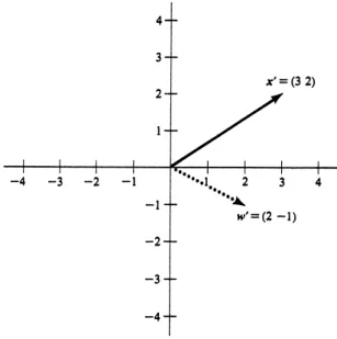
- Geometric Interpretations of Vectors
- Linear Equations and Solutions
- Orthogonal Transformations and Projections
- Eigenvalues and Eigenvectors
- Singular Value Decomposition
- Summary
- Exercises
The sum of the squares of the elements in the column vectorx is given by (matrix multiplication)xx. This solution is unique only if r(A) is equal to the number of unknowns in the set of equations. A computer is used to obtain generalized inverses when necessary.). The proportion of the total sum of squares represented by the first principal component is λ1/.
MULTIPLE REGRESSION IN MATRIX NOTATION
The Model
The definition of each partial regression coefficient is dependent on the set of independent variables in the model. Since the random vector is assumed to be independent of each other, the covariance between Since the elements of X and β are assumed to be constants, the Xβ TheY vector expression in the model is a vector of constants.
The Normal Equations and Their Solution
A review of the normal equations in Chapter 1, Equation 1.6, reveals that the elements in this 2×2 matrix are the coefficients on β0 and β1. The reader can verify that these are the right-hand sides of the two normal equations, Equation 1.6. Only two allelic frequencies should be reported; the third is redundant as it can be calculated from the first two and the ones column.
The Y and Residuals Vectors
Recall that least squares estimation minimizes the sum of squares of the residuals; β is chosen so that it is a minimum.
Properties of Linear Functions of Random VectorsVectors
The ith diagonal element of AA is the sum of the squares of the coefficients (aiai) of the ith linear functionui =aiZ. The (i,j)th off-diagonal element is the sum of the products of the coefficients (aiaj) of the ith and jth linear function and, when multiplied by σ2, gives the covariance between two linear functions sui=aiZanduj=ajZ. Note that it is the sum of the squares of the coefficients of the linear function a2i, which is the result given in Section 1.5.
Properties of Regression Estimates
If important independent variables are omitted or if the functional form of the model is incorrect, Xβ will not be the expectation of Y. The variances and covariances of the estimated regression coefficients are therefore given by the elements of (XX)−1 multiplied by σ2. The variance of each Yi is therefore always smaller than σ2, the variance of the individual observations.
Summary of Matrix Formulae
The smaller variance of the residuals for the points far from the "center of the data" indicates that the fitted regression line or response surface tends to get closer to the observed values for those points. In designed experiments, the levels of the independent variables are subject to the researcher's control. Thus, except for the magnitude of σ2, the precision of the experiment is under the researcher's control and can be known before the experiment is run.
Exercises
Show that the regression equation obtained using centered data is equivalent to that obtained using the original uncentered data. Another method to take into account the experience of non-smokers is to use X2= ln(number of hospital days for non-smokers) as an independent variable. a) Set X and β for the regression of Y = ln(number of hospital days for smokers) on X1 = (number of cigarettes)2 and Set up the regression problem to determine whether the discrepancy Y is related to any of the four independent variables.
ANALYSIS OF VARIANCE AND QUADRATIC FORMS
Introduction to Quadratic Forms
Therefore, the sum of squares due to correction for the mean has 1 degree of freedom. The sum of squares resulting from the linear regression on temperature is given by the quadratic form. The defining matrix A2 is idempotent with tr(A2) = 1 and therefore the sum of squares has 1 degree of freedom.
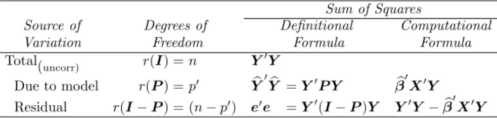
Analysis of Variance
It is the residual sum of squares after fitting the model and is labeled SS(Res). SS(Regr) = SS(Model)−SS(µ), (4.19) where SS(Model) is understood as the sum of squares due to the model containing the independent variables. The sum of squares due to µ alone, SS(µ), is determined using matrix SS(µ) notation to show the evolution of the defining matrices for .
Expectations of Quadratic Forms
The regression mean square MS(Regr) is an estimate of σ2 plus a quadratic function of all βje except β0. Comparison of MS(Regr) and MS(Res) therefore provides the basis for judging the importance of the regression coefficients or equivalently of the independent variables. From equation 4.33 it can be seen that MS(Res), in such cases, will be a positively biased estimate of σ2.
Distribution of Quadratic Forms
The scale in each case is division of the chi-squared random variable by its degrees of freedom. The noncentrality parameter of the chi-square distribution is the second term of the expectations of the quadratic forms divided by 2 (see equation 4.25). All the quantities except β in the noncentrality parameter are known before the experiment is carried out (in those cases where the X's are subject to the control of the researcher).
General Form for Hypothesis Testing
The null hypothesis is violated if any one or more equalities in H0 are not true. The variance is obtained by applying the rules for the variances of linear functions (see Section 3.4). The sum of squares for the linear hypothesis H0:Kβ= is the sum of squares incorrectly calculated by [see Searle.
A simple hypothesis
- Univariate and Joint Confidence Regions
- Estimation of Pure Error
- Exercises
The successive sum of squares for X2 is SS(Regr) for this model minus SS(Regr) for the first model and is given in R notation by R(β2|β0 β1). The four independent variables are described in Exercise 3.12. a) The first model used the cross section and all four independent variables. i) Calculate SS(Model), SS(Regr) and SS(Res) for this model and summarize the results in the analysis of variance table. ANALYSIS OF VARIANCE AND QUADRATIC FORMS. estimated average seed weight for average radiation level and 0.07 ppm ozone.

CASE STUDY: FIVE
INDEPENDENT VARIABLES
Spartina Biomass Production in the Cape Fear Estuary
Subsoil samples from 5 random sites within each location-vegetation type (giving a total of 45 samples) were analyzed for 14 soil physicochemical characteristics every month for several months. The purpose of this case study is to use multiple linear regression to relate total variability in Spartina biomass production to total variability in five substrate variables. It is left as an exercise for the student to study separately the relationships indicated by variation among vegetation types and locations (using the location-vegetation-type tools) and the relationships indicated by variation among samples within location-vegetation-type combinations.
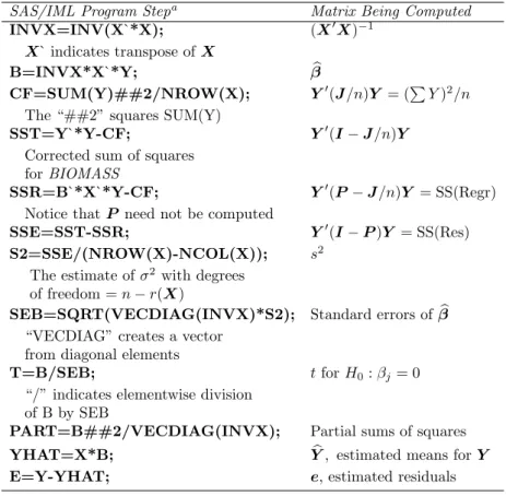
Regression Analysis for the Full Model
The first row of ρ contains the simple correlations of the dependent variable with each of the independent variables. The results of the multiple regression analysis using all five independent Summary of Results variables are summarized in Table 5.2. Thus, 68% of the sums of squares in BIOMASS can be associated with the variation in these five independent variables.
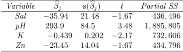
Simplifying the Model
For this example, one variable is eliminated at a time: the one whose elimination will cause the smallest increase in the remaining sum of squares. The variable Na has the smallest partial sum of squares in the five-variable model. Because the partial sums of the squares for both pH and Kar are significant, the simplification of the model stops at this model with two variables.
Results of the Final Model
This shows that the two-dimensional confidence ellipse is not a projection of the three-dimensional confidence ellipsoid. The general shape of the confidence zone can be seen from the three-dimensional image. Intersection of Bonferroni confidence intervals (inner box) and intersection of Scheff´e confidence intervals (outer box).

General Comments
The predicted change in BIOMASS per unit change in pH ignores all variables not included in the final prediction equation. The partial regression coefficients are the slopes of the response surface in the directions represented by the corresponding independent variables. This requires that the values of the independent variables for the prediction points must be in the sample space.
Exercises
Construct a joint 95% confidence interval for the partial regression coefficients for X8 and X9 without considering the parameters for the other variables in your final model in Exercise 5.4.
GEOMETRY OF LEAST SQUARES
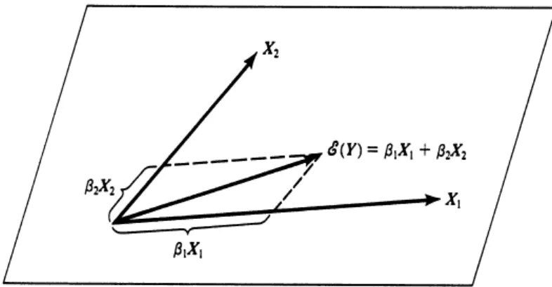
Linear Model and Solution
The dotted lines in Figure 6.1 show the addition of the vectors β1X1 and β2X2 to give the vector E(Y). The signs of β1 and β2 are determined by the region of X-space in which Y falls, as illustrated in Figure 6.2 for β1 and β2. The closest point on the plane to Y (in Figure 6.3) is the point that would be reached by a plumb line.