An example of this development is the publication this year of the ASM handbook on CD-ROM. Before acknowledging contributors to this volume, it is important to acknowledge the excellent work of the editors of the first edition: Timothy L. Piwonka (University of Alabama) authored the "Casting" section. Tom also served as Section Chair and contributing author to Casting, Volume 15 of the ASM Handbook, published in 1988.
Blau (Oak Ridge National Laboratory) authored the article "Wear Testing." Peter also served as binding coordinator for Friction, Lubrication, and Wear Technology, volume 18 of the ASM Handbook, published in 1992. Erhard also served as binding coordinator for Powder Metallurgy, volume 7 of the ASM Handbook, published in 1984. Additional source information can be found in the reference lists, that appears in many of the articles.
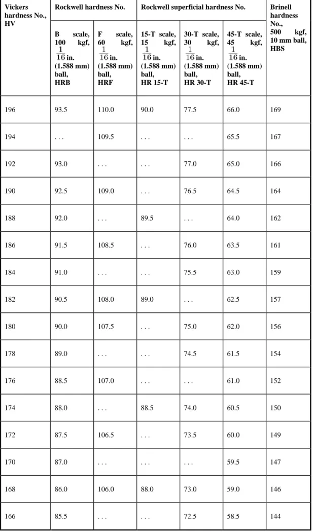
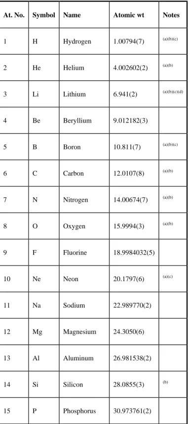
Davis; prepared under the direction of the ASM International Handbook Committee.-- Desk ed.; 2nd edition. Unit conversion factor. a) The numbers in brackets are the uncertainties of one standard deviation in the last digits of the stated value, calculated by internal consistency. Significant deviations in the atomic weight of the element from that given in the table can occur.
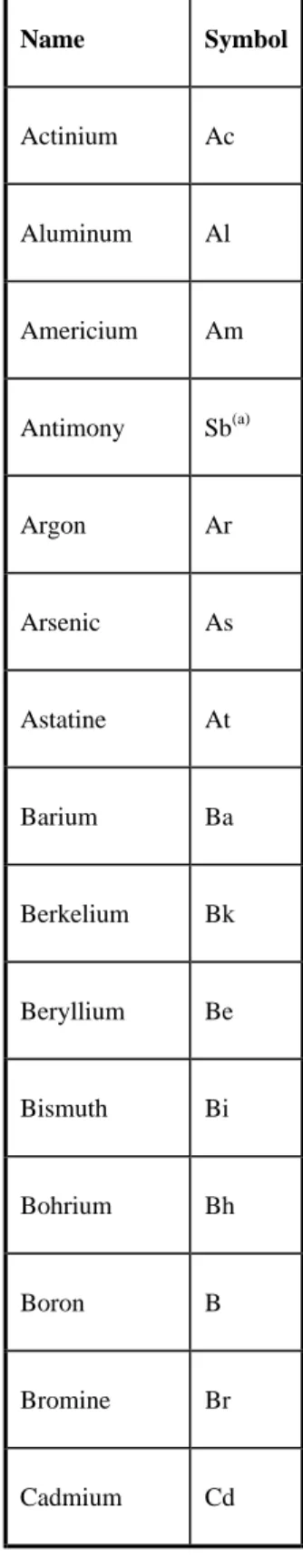
Those elements that do not exhibit the characteristics of the metallic elements are called nonmetals (see the periodic table).
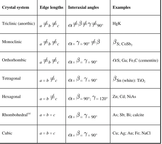
Crystal Structure of Metallic Elements
Introduction
Crystallographic Terms and Basic Concepts
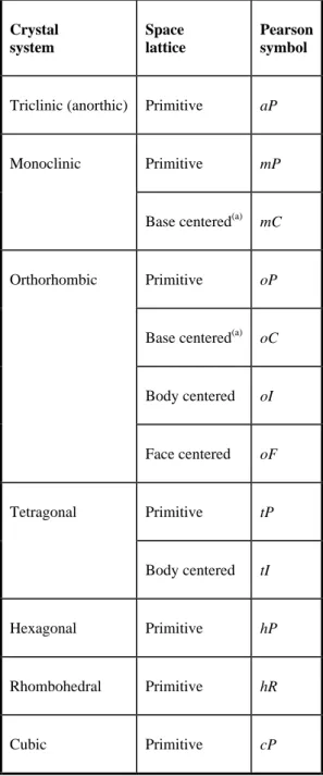
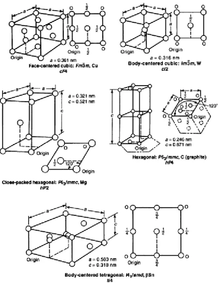
When the edges of the unit cell are not equal in all three directions, all unequal lengths must be stated to completely define the crystal. The first four are: primitive (simple), with grid points only at cell corners; base plane centered (end centered), with grid points centered on the C planes, or ends of the cell; all planes centered, with grid points centered on all planes; and in-centered (body-centered), with grid points at the center of the volume of the unit cell. A truer representation of the effective diameters of the atoms in a unit cell is shown in Fig.
It consists of the space lattice symbol followed by letters and numbers indicating the symmetry of the crystal. The lattice parameter of the unit cells is taken to be exactly ±2 in the last digit reported. 7 AuCu II structure; a one-dimensional long-period superlattice, with antiphase boundaries spaced at intervals of five unit cells in the disordered state.
Crystal Defects and Plastic Flow
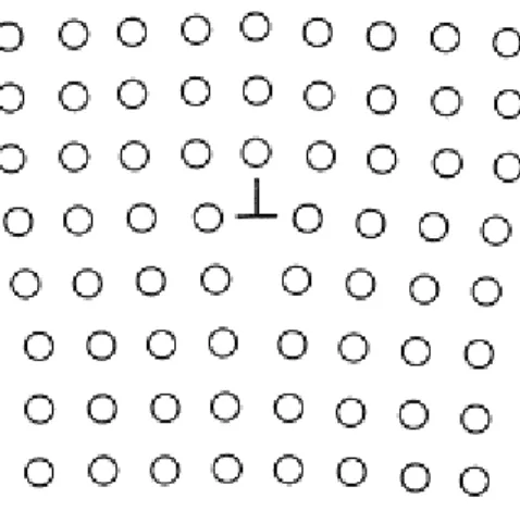
9 A section through an edge offset, which is perpendicular to the plane of the illustration and is indicated by the symbol. The part of the line on the left near the front of the crystal and perpendicular to the arrows, in Fig. The part of the slip zone near the right side, where the displacement is parallel to the dislocation, is called a screw dislocation.
As the slipped region spreads across the slip plane, the edge-type portion of the dislocation moves out of the crystal, leaving the screw-type portion still embedded, as shown in Fig. When all the dislocations finally come out of the crystal, the crystal will be perfect again, but with the upper part displacing one unit cell from the lower part, as shown in Fig. 12 Small-angle boundary (subboundary) of the tilt type, which consists of a vertical series of edge shifts.
Alloy Phase Diagrams and Microstructure
The twin relationship may be such that the lattice of one part is the mirror image of the other part, or one part may be related to the other by some rotation about a particular crystallographic axis. Twin boundaries are generally very flat and appear as straight lines in photomicrographs and are two-dimensional defects with lower energy than high-angle grain boundaries. Twin boundaries are therefore less effective as sources and sinks for other defects and are less active in deformation and corrosion than ordinary grain boundaries.
The plastic deformation of a metal at a temperature at which annealing does not proceed rapidly is called cold working, and this temperature depends mainly on the metal in question. As the amount of cold working increases, the distortion caused in the internal structure of the metal makes further plastic deformation difficult, and the strength and hardness of the metal increase.
Common Terms
Growth twins can often occur during crystallization from the liquid or vapor state, by growth during annealing (by recrystallization or by grain growth processes), or by movement between solid phases, such as during phase transformation. In a phase diagram, however, each single-phase field (phase fields are discussed in a later section) is usually given a single label, and engineers often find it convenient to use this label to refer to all materials within the field . regardless of how continuously the physical properties of materials vary from one part of the field to another. A physical system consists of a substance (or group of substances) that is isolated from its surroundings, a concept used to facilitate the study of the effects of state conditions.
For example, the substances in alloy systems can be two metals such as copper and zinc; a metal and a non-metal such as iron and carbon; a metal and an intermetallic compound such as iron and cementite;. A single-component phase diagram can simply be a one- or two-dimensional plot showing the phase changes in the substance as temperature and/or pressure change. Willard Gibbs in 1876, relates the physical state of a mixture to the number of constituents in the system and to its conditions.
Unary Diagrams
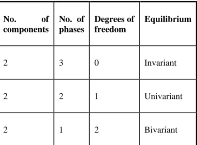
The phase rule says that a stable equilibrium between two phases in a unary system allows one degree of freedom (f). This state, called univariant equilibrium or monovariant equilibrium, is illustrated as lines 1, 2, and 3 that represent the single-phase fields in Fig. Once a pressure is selected, there is only one temperature that satisfies the equilibrium conditions, and vice versa.
The three curves starting from the triple point are called triple curves: line 1, representing the reaction between the solid phase and the gas phase, is the sublimation curve; line 2 is the melting curve; and line 3 is the evaporation curve. The evaporation curve ends at point 4, called a critical point, where the physical distinction between the liquid and gas phases disappears. If both the pressure and the temperature in an unary system are freely and arbitrarily chosen, the situation is equivalent to having two degrees of freedom, and the phase rule states that only one phase can exist in stable equilibrium (p.
Binary Diagrams
When this occurs in a binary system, the phase diagram usually has the general appearance of that shown in Fig. If the solidus and liquidus meet tangentially at a point, a maximum or minimum is produced in the two-phase field, dividing it into two portions as shown in Fig. It is also possible to have a mixing gap in a single-phase field; this is shown in Fig.
6 Binary phase diagrams with invariant points. a) Hypothetical diagram as shown in Figure 5, except that the miscibility gap in the solid touches the solidus curve at the invariant point P; an actual diagram of this type probably does not exist. When this happens, the liquidus and solidus curves (and their expansion into the two-phase field) for each of the final phases (see Fig. 6c) resemble those for the situation of complete miscibility between the system components shown in Fig. These and other different types of invariant reactions observed in binary systems are listed in Table 1 and shown in Fig.
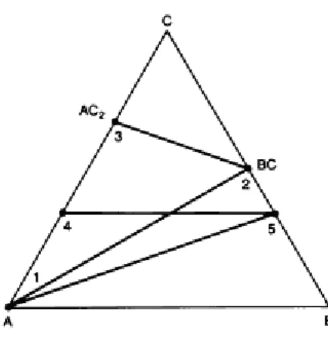
Ternary Diagrams
When the components of the system are metallic, such an intermediate phase is often called an intermetallic compound. A common pseudobinary section is one in which the percentage of one of the components is kept constant (the section is parallel to one of the faces), as shown by lines 4-5 in Fig. Another is one in which the ratio of two constituents is kept constant and the amount of the third is varied from 0 to 100% (lines 1–5).
Therefore, contour lines of equal temperature (isotherm) are often added to the projected views of these surfaces to indicate the shape of the surfaces (see Fig. 12). The sum of a system's kinetic energy (kinetic energy) and potential energy (stored energy) of a system is called its internal energy, E. Thermal energy changes under constant pressure (again neglecting field effects) can most easily be expressed in terms of the enthalpy, H, of a system.
Thermodynamics and Phase Diagrams
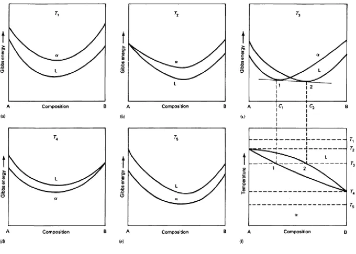
For a spontaneous (irreversible) process, the change in Gibbs energy is less than zero (negative); that is, the Gibbs energy decreases during the process and it reaches a minimum at equilibrium. 13 Using Gibbs energy curves to construct a binary phase diagram showing miscibility in both liquid and solid states. At temperature T1, the liquid solution has the lower Gibbs energy and is therefore the more stable phase.
If the Gibbs energy curves for the liquid and the solid at a certain temperature become tangential at a certain point, the resulting phase diagram will be similar to that shown in Fig. Eutectic phase diagrams are shown, a feature of which is a field where there is a mixture of two solid phases, can also be constructed from Gibbs energy curves. Similarly, Gibbs energy surfaces and tangential planes can be used to construct ternary phase diagrams.
Reading Phase Diagrams
Metallography and Microstructures, Vol 9, 9th ed., ASM Handbook, ASM International, 1985 Examples of Phase Diagrams
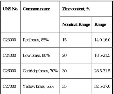
Alloys at the high copper end (red brass, low brass, and investment brass) lie in the solid solution copper phase field and are called brasses after the old designation for that field. As expected, the microstructure of these brasses consists exclusively of copper solid solution grains (see Fig. 27a). The stress on the copper crystals caused by the presence of zinc atoms causes solution hardening in the alloys.
As a result, the strength of the brasses, both in the work-hardened and annealed condition, increases with increasing zinc content. Therefore, the microstructure of these so-called α-β alloys shows different amounts of β phase (see Figs 27b and 27c), and their strengths are further increased relative to that of the α-brass. Although the phase diagram of this system is quite complex (see Fig. 28), the alloys of interest in this discussion are confined to the region on the aluminum side of the diagram where a simple eutectic is formed between the aluminum solid solution and the θ (Al2Cu) phase.