They represent a modification of Biot1 theory in that they include explicit temperature dependence, and a thermodynamically consistent incorporation of the time-temperature superposition principle for treating media with temperature-dependent viscosity coefficients. To complement the theoretical development provided in Part I, let us consider certain aspects of the theories proposed by Biot and SOITle by other researchers relating to the treatment of. The initial Biot formulation (1) allowed the thermodynamic system to have a non-uniform temperature distribution, but temperature variations were treated as hidden coordinates (that is, the temperature at the geometric boundary of the system was set to a constant reference temperature held). .
Another limiting assumption introduced in his formulation is that the viscous properties of the system are independent of temperature. Recently, Hunter (6) and Chu (7) have directly addressed the derivation of the stress-strain temperature equations and the associated energy equation of isotropic, viscoelastic solids. The situation in which this Voigt or Maxwell representation is not thermodynamically admissible only occurs when the temperature is transient and the viscous properties of the material are such that the time-temperature superposition principle (9, p. 209) does not is complied with.
Provided that the time-temperature superposition principle is applicable, there is another interesting implication of thermodynamic analysis.
GENERAL THEORY
Since the combined system consisting of the reservoir and the real system is isolated, the entropy change of the reservoir is dS. The basic thermodynamic equations 1.33 will now be solved to obtain q. as an explicit function of the thermal and mechanical loading. In view of the generality and simplicity embodied in the operational notation in 1.37, we will use it throughout this thesis. and.
This minimal character of V T In the neighborhood of the reference state exists of course also when. These equations are of the same form as equations 1.33 which are derived for a system at a defined point, 1J With this last assumption, all the results of Section 1.3 are applicable to the solution of Equations 1.98 after setting F = 1,.
4 after linearizing the energy equation (see Eqs. 1.71 and 1.72) is consistent with the results of the present.
APPLICATIONS TO VISCOELASTIC SOLIDS
For a complete description of the thermomechanical behavior of viscoelastic solids it is necessary to include the equations of strain-displacement, mechanical equilibrium and heat conduction together with the stress-strain-temperature and energy equations considered above. Because of the second term appearing in equation 1.122, this transformation mayor may not simplify the calculation depending on the specific application. This section deals with the role of the rrriodynamics in problems of finite viscoelastic deformation and crack propagation.
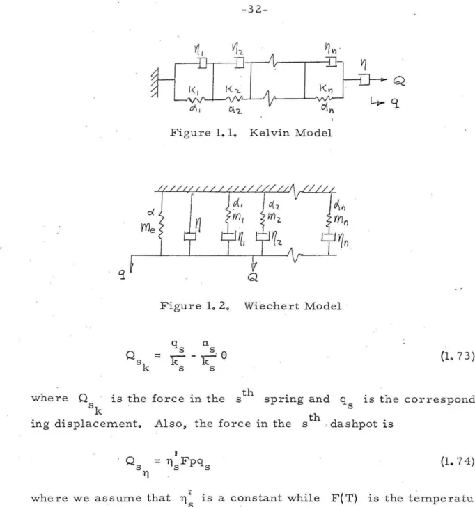
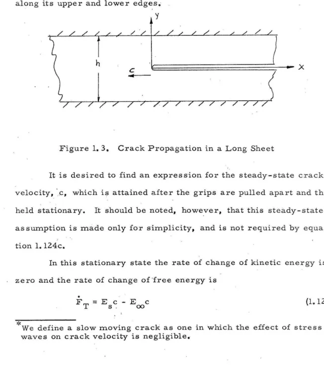
Indeed, if the imposed strain rates are not too high, it is reasonable to assume that the linear rate law loll applies regardless of the magnitude of strain. 4, in which the actual (dashed lines) shape is approximated by the solid, straight lines, and the distance L can be a function of the crack speed c. The dissipation will be calculated using the general Wiechert ITlodel, figure 1.2, (but without the free dashpot, ,) to calculate the. uniaxial tensile response of the plate.
The dissipation per unit of volume is given by the steady-state transformation, cit - c dx ' such that.
PART II
However, one of the purposes of this chapter is to show that the general equations for linear systems are the Euler equations for a variational principle, which is analogous to Hamilton's principle, in that it consists of a time integral which has a certain thermodynamic meaning. It will be seen that all the functionals can be derived directly from the thermodynamic fundamentals by calculating the appropriate free energy and dissipation functions. By applying the coordinate principle, we thus arrive at a variation principle for the entropy displacement field, while application of the complement theorem leads to a temperature-related one.
Biot (2) has indicated that equation 2.1 can be obtained from an operational variational principle in which an operational form of the dissipation function is introduced as. Before proceeding with the statement of the theorem, some observations will be made regarding the term Qj. Therefore, based on the above relationship between IQ and I, we expect the Euler equations of.
Comparing this with equations and 2.10, the generalized free energy density V (per unit volume) is defined as. which can also be expressed as a function of temperature using the energy equation 2. We note that the dissipation density is D. or, depending on the temperature, I in the general theory can now be written by substituting the equation q. where Ae is the part of the surface on which e = e is prescribed, and S.n. The same complementary property can be expected in other applications as a consequence of the fact that the basic thermodynamic equations of motion are the same for all linear systems.
67, and heat conduction equation 2.36; based on this comment as well as the fact that the natural boundary conditions of the variation are 2.72. In light of the comments on the general principles in section 2.2, the variation principle 2.72 can be formulated in terms of the. This will show more clearly the close correspondence between the basic form of the variational principle given in section 2.
In addition, the natural boundary conditions of the variation are the conditions in the Lagrang multiplier.e. Thus, the functional's transformation into Reissner's. principle, equation 2.103, is simply stationary on the positive real axis p. It is well established that these equations are the complete, correct set for describing the displacement and temperature distribution.
The necessary modifications are determined by examining the effect of the temperature on the Euler equations and boundary conditions.
PART III
This analysis is then used in a discussion of the relationship between errors in approximate and exact viscoelastic and elastic solutions. For example, it is known a priori that all the singularities of Laplace-transformed solutions are on the non-p 0 positive real axis. P and is the transformed displacement vector. but the matrix consisting of the sum of those in 3.
It is noted that the singularities of Q/3 are simple poles (or branches if P = P (x,)) on the negative real p-axis, but if the. boundary conditions all relate to tension, Q/3 Also for the symmetry of They we have. The tional moduli in equations 3.15' are left in the volume integrals because properties cannot be functions of x. The order of the poles of qa can be determined by examining the behavior of q in combination with equation 3.23 as p approaches. It can be shown that stresses derived from the transformed coherent principle have a similar dependence as those of the displacements discussed above.
1J J. to the prescribed surface .force, T io It is further assumed that for each a l~) satisfies the equilibrium equations. H(t) satisfies the equilibrium equations with pre- 1J. The Laplace transform of the complementary functional, Equation 2.94, is neglected for two temperatures. simplicity). Since this leads to an infinite (delta function) stre s s at t = 0. we will exclude this in all the following work by acidizing.
However, theorem II and reg.uire, except for the restriction mentioned above, that the finite sum representation I of the stress-strain relations be used. Postulate, II - ' The most time dependence ra1 of genes of generalized coordinates is. butions of the variable '7 which ITconsists of. wholly or .partially of the Dirac-delta functions. It is clear that the finite degree free cases considered in Sections 3.2b are obtained immediately by setting
The time dependence of QI3 is immediately obtained from the Stieltjes transformation theory (32) (an assumption of some rea'E;onable convergence, properties of the improper integrals), and it turns out to be the same / as given by equation 3. It is clear that the error estimate, Equation 3.51, cannot actually be used in practice, as it requires knowledge of an exact solution.
PART IV
6 and the resulting expression is written in terms of the original functions tj;(t). Due to the skewed shape of the weighting function, a somewhat better formula was found to be. Third, the accuracy of the inversion can be improved by adding more terms to the series.
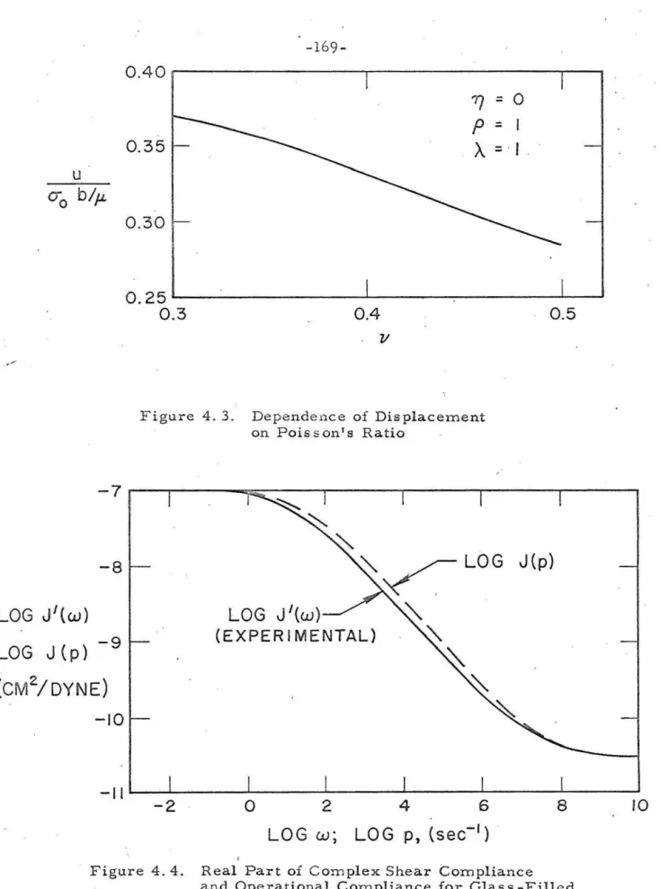
Based on the correspondence rule, this procedure yields the approximate transformed viscoelastic solution. It is also required, based on the symmetry in this problem, that f is an odd function of p, while g is even. To illustrate the calculation of the viscoelastic solution, it is sufficient to consider only the u displacement with T]::: 0, P = 1, A.:::.
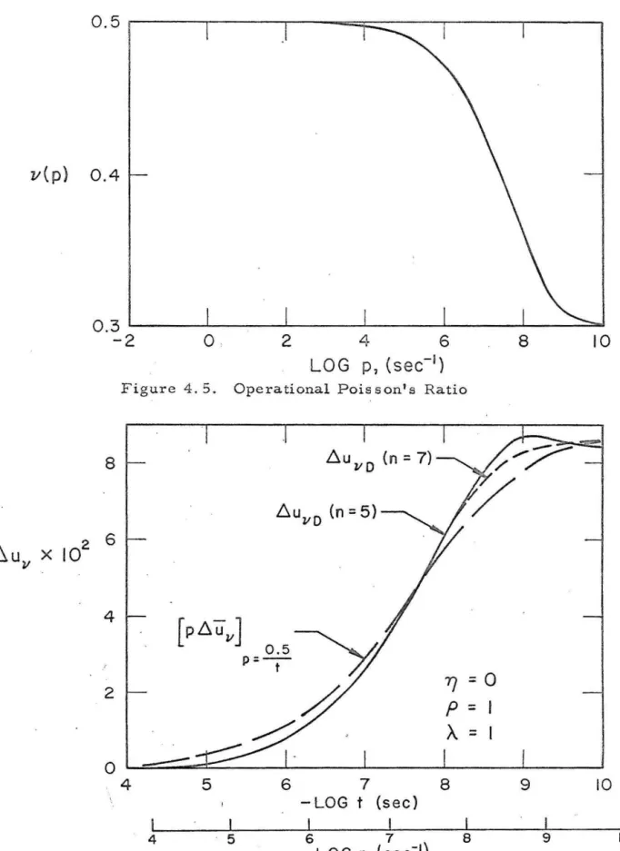
But since one of our goals is to illustrate the simplicity of approximate inversion methods by inverting the transformation. which is a very involved function of material properties, we will find out. Because of the relative size of the matrix elements, this system can be easily solved by iteration to obtain the time dependence. It is clear that the poles of v(p) appear only when the denominator vanishes and that these are simple poles, since the derivative of the denominator does not vanish in the finite p-plane.
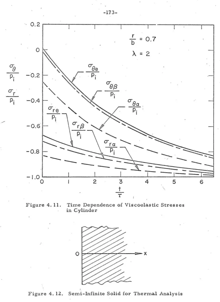
On the basis of the correspondence rule, the time-dependent stresses are obtained by replacing Poisson's ratio,. 73 and the variations, a system of linear algebraic equations is obtained for determining the constants Ca'. It can be shown that the matrix of coefficients which multiplies C is symmetric;. Namely, the class for which the assumed solution is a non-linear function of the unspecified generalized coordinates.
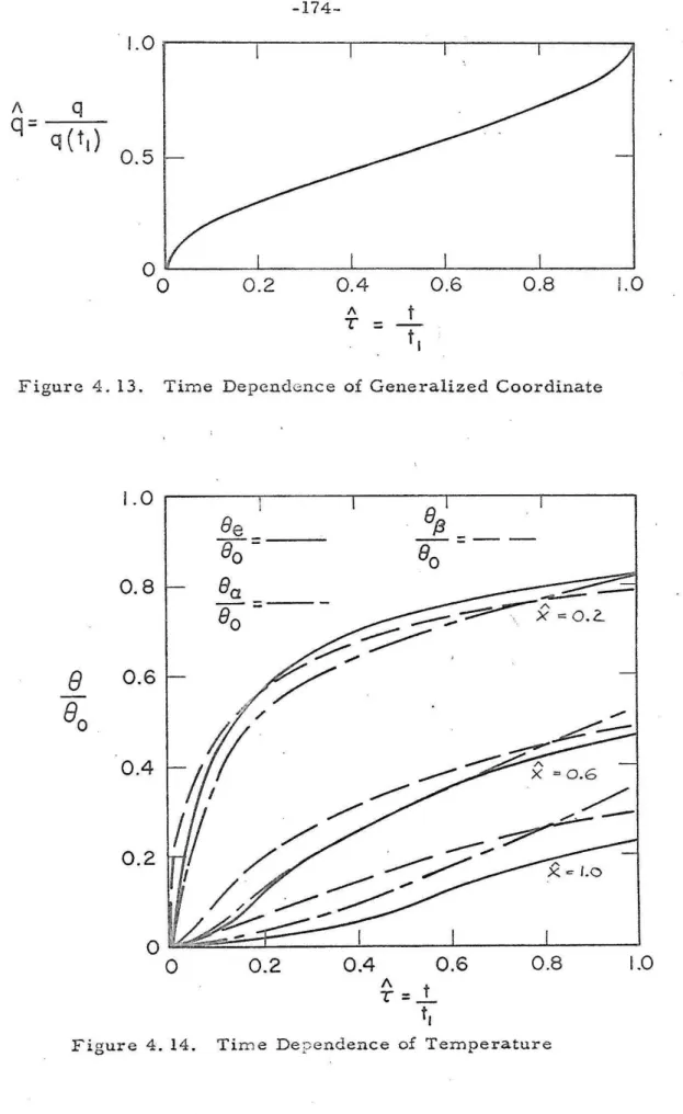
This approximate solution is shown in Figure 4.14 together with the exact temperature, which given the variables ;; and r is. American Mathematical Society Symposium on the Calculus of Variations and Its Applications (April 12, 1956).
8 LOG J'(w)
R2 (CONTOUR