Can bank be a source of contagion during the 1997 Asian crisis?
Chu-Sheng Tai
*Department of Economics and Finance, College of Business Administration,
Texas A&M University-Kingsville, MSC 186, 700 University Blvd., Kingsville, TX 78363-8203, USA Accepted 24 February 2003
Abstract
This paper tests whether bank can be a source of contagion during the 1997 Asian crisis using asset return data from a crisis country – Thailand. In particular, I examine whether Thai banking sector can produce contagion effects in both conditional means and volatilities of its foreign exchange and stock markets during the crisis after controlling economic fundamentals.
The test results show that contagion-in-mean effects appear to be multidirectional since return shocks emanating from any one of the three markets can sweep across all markets, but contagion-in-volatility effects are mainly driven by the negative return shocks originating in the banking sector. Overall the empirical evidence indicates that the past return shocks ema- nating from banking sector have significant impact not only on the volatilities of foreign exchange and aggregate stock markets, but also on their prices, suggesting that bank can be a major source of contagion during the crisis.
2003 Elsevier B.V. All rights reserved.
JEL classification:C32; F31; G12
Keywords:Bank; Contagion; Spillover; Risk premium; Multivariate GARCH-M
1. Introduction
It is well-known that equity, currency, and banking crises cannot only generate substantial real costs for the country in which they occur, but also spill over to other countries and exacerbate the problem. The financial crisis of East Asia in 1997 was
*Tel.: +1-361-593-2355; fax: +1-361-593-3912.
E-mail address:[email protected](C.-S. Tai).
0378-4266/$ - see front matter 2003 Elsevier B.V. All rights reserved.
doi:10.1016/j.jbankfin.2003.02.001
www.elsevier.com/locate/econbase
largely unanticipated and was characterized by sharp falls in currency values and stock prices in several countries simultaneously. A number of complex factors trig- ged the financial crisis in East Asia, but, fundamentally, unbridled expansion and subsequent contraction of banking lending played a leading role. Kaminsky and Reinhart (1999) systematically analyze the links between banking and currency crisis and document that problems in the banking sector typically precede a currency cri- sis. One of the biggest challenges facing scholars studying the East Asian financial crisis is to explain this contagion in which crisis emanating from one country soon swept across all countries in the region.
There are number of reasons why banking centers may add to financial contagion.
These can be classified into two types of financial contagion (see Van Rijckeghem and Weder, 1999). The first has been called the ‘‘common bank lender channel’’.
Due to the increasing cross-border integration among banks, a common lender can be the main source of funds for several countries. But, competition for funds from the same bank might become a problem. For example, consider the case in which the firms from two countries A and B borrow from the same banking system (say, country C). When a crisis hits A, banks from C may face defaults on loans to A.
To restore capital adequacy ratios, country C can provoke a credit crunch in country B by calling in the loans. Thus, the productive sector of country B comes under pres- sure and eventually the whole country may face a crisis. In this case, even if B’s econ- omy is not directly linked to A’s, the presence of a third party C makes the crisis spread from one country to the other. The second kind of contagious response also leads to outflows but, in contrast with the common lender channel there is no need for a real linkage through losses. In other words, even if banks had no exposure in the primary crisis country they might still react with a generalized reduction of credit to other countries, due to revisions of expected returns in this asset class or a general- ized increase in risk-aversion. This financial contagion due to common bank lenders will not be considered as ‘‘pure contagion effect’’ according to Masson (1998). In stead, it will be categorized as ‘‘spillover effect’’ due to financial interdependence. 1 However, the second type of financial contagion can be qualified as the pure conta- gion effect because the transmission of financial crises is not due to financial interde- pendence and neither can it be explained by changes in fundamentals.
This goal of this paper is to test whether bank can be a source of contagion during the 1997 Asian crisis using asset return data from a crisis country – Thailand. In par- ticular, I examine whether Thai banking sector can produce contagion effects in both conditional means and volatilities of its foreign exchange and stock markets during the crisis. Previous studies on contagion have failed to take into account the impor-
1This spillover effect may also result from trade linkages. Another channel that financial markets turbulence can spread from one country to another according to Masson (1998) is ‘‘monsoonal’ effects, or Ôcontagions from common causes’, which tend to occur when affected countries have similar economic fundamentals or face common external shocks. Masson (1998) categorizes these two channels of financial crisis as fundamentals-driven crises since the affected countries share some macroeconomic fundamentals, which implies that the transmission of financial crises is due to the interdependence among those countries and not necessarily due to contagion.
tant distinction between the two concepts of interdependence and contagion. Specif- ically, in this paper I defineÔcontagion’ as significant spillovers of asset-specific idio- syncratic shocks during the crisis after economic fundamentals or systematic risks have been accounted for. In testing for contagion, its existence depends on the eco- nomic fundamentals used. Unfortunately, there is disagreement on the definitions of the fundamentals. To control for the economic fundamentals, most empirical studies tend to choose those fundamentals arbitrarily, such as by using macroeconomic vari- ables, dummies for important events, and time trends. The problem with these con- trol variables is that contagion is not well defined without reference to a theory. To overcome this problem, I rely on an international capital asset pricing model (ICAPM), which provides me a theoretical basis in selecting the economic funda- mental. The economic fundamental under ICAPM is the world market risk, so the evidence of contagion is based on testing whether idiosyncratic risks – the part that cannot be explained by the world market risk, are significant in describing the dynamics of conditional means and volatilities of foreign exchange and stock mar- kets during the crisis period.
In addition to the contribution in overcoming the drawback of arbitrarily choos- ing economic fundamentals in testing contagion in previous studies, another contri- bution of this paper is methodology used to test contagion. In particular, I utilize an asymmetric Multivariate General Autoregressive Conditional Heteroscedastic in Mean (MGARCH-M) approach to model conditional mean and asymmetric volatil- ity spillovers during the crisis, in addition to capturing the time dependencies in the second moments of asset returns, a stylized property found in most financial time- series, which has been ignored by most empirical studies on contagion.2Therefore, under the fully parameterized multivariate model adopted in this paper, not only is the maximum efficiency gain retained in controlling the systematic risks when testing the contagion, but also some interesting statistics are recovered, which are mostly ignored in previous studies.
The test results show that contagion-in-mean effects appear to be multidirectional since return shocks emanating from any one of the three markets (banking sector, foreign exchange, and stock markets) can swept across all markets, but contagion- in-volatility effects are mainly driven by the negative return shocks originating in
2According to Forbes and Rigobon (1999), Dornbusch et al. (1999), and Kaminsky and Reinhart (2000), previous empirical studies on contagion can be categorized by methodology into four groups: (1) the testing of significant increases in correlation (Calvo and Reinhart, 1996; Baig and Goldfajn, 1999;
Forbes and Rigobon, 1998, 1999; Park and Song, 1999); (2) the testing of significance in innovation correlation (Baig and Goldfajn, 1999); (3) the testing of significant volatility spillover (Edwards, 1998;
Edwards and Susmel, 1999); (4) crisis prediction regression (Bae et al., 2000; Eichengreen et al., 1996;
Kaminsky and Reinhart, 2000; Van Rijckeghem and Weder, 1999; Sachs et al., 1996). None of the contagion studies mentioned above explicitly takes the time dependencies in the second moment into account. A recent paper by Bekaert et al. (2005, forthcoming) applies three-stage univariate GARCH model to study contagion in equity markets by testing whether there is evidence of significant increase in cross-market residual correlation during the crisis. Although they model conditional second moments, they cannot answer whether return shocks originated from one market will significantly affect the other markets during the crisis.
the banking sector. This empirical finding indicates that not only can bank return shocks become contagious at volatility level, but they can also become contagious at mean level, suggesting that bank can be a major source of contagion during the crisis.
The remainder of the paper is organized as follows. Section 2 presents the theo- retical asset-pricing model used to control for systematic risks when testing pure con- tagion effects. Section 3 describes the econometric methodology employed to estimate the model and several test hypotheses are presented in Section 4. Section 5 describes the data and empirical results are reported in Section 6. Some conclusions are offered in the final section.
2. The theoretical motivation
We know that the first-order condition of any consumer-investor’s portfolio opti- mization problem can be written as
E½MtRi;tjXt1 ¼1; 8i¼1;. . .;N; ð1Þ
whereMt is known as a stochastic discount factor (SDF) or an intertemporal mar- ginal rate of substitution (IMRS);Ri;tis the gross return of assetiat timetandXt1is market information known at timet1. Without specifying the form ofMt, Eq. (1) has little empirical content since it is easy to find some random variableMtfor which the equation holds. Thus, it is the specific form of Mt implied by an asset pricing model that gives Eq. (1) further empirical content (e.g., Ferson, 1995; Tai, 2000).
SupposeMt andRi;thave the following factor representations:
Mt¼aþXK
k¼1
bkFk;tþut; ð2Þ
ri;t¼aiþXK
k¼1
bikFk;tþei;t 8i¼1;. . .;N; ð3Þ
whereri;t¼Ri;tR0;tis the raw returns of assetiin excess of the risk-free rate,R0;t, at time t, and E½utFk;tjXt1 ¼E½utjXt1 ¼E½ei;tFk;tjXt1 ¼E½ei;tjXt1 ¼0 8i;k; Fk;t are common risk factors which capture systematic risk affecting all assets ri;t including Mt; bik are the associated time-invariant factor loadings which measure the sensi- tivities of the asset to the common risk factors, whileutis an innovation andei;t are idiosyncratic terms which reflect unsystematic risk. The risk-free rate, R0;t1, must also satisfy Eq. (1).
E½MtR0;t1jXt1 ¼1: ð4Þ
Subtract Eq. (4) from Eq. (1), we obtain
E½Mtri;tjXt1 ¼0 8i¼1;. . .;N: ð5Þ
Apply the definition of covariance to Eq. (5), obtaining E½ri;tjXt1 ¼Covðri;t;MtjXt1Þ
E½MtjXt1 8i¼1;. . .;N: ð6Þ
Substitute Eq. (2) into Eq. (6):
E½ri;tjXt1 ¼X
k
bk
E½MtjXt1Covðri;t;Fk;tjXt1Þ
¼X
k
kk;t1Covðri;t;Fk;tjXt1Þ; ð7Þ
wherekk;t1 is the time-varying price of factor risk. Eq. (7) is a general conditional multifactor asset-pricing model derived from the intertemporal consumption- investment optimization problem.
In empirical tests, the SDF is projected onto the world market portfolio. That is, I extend the domestic CAPM into an international setting.3Therefore, a conditional international CAPM (ICAPM) will be used to control for systematic risk in testing contagion. I can now rewrite the conditional asset-pricing model in Eq. (7) as
ri;t¼kw;t1Covðri;t;rw;tjXt1Þ þei;t 8i¼1;. . .;N; ð8Þ where ‘‘w’’ denotes world market risk.
3. Econometric methodology
The conditional ICAPM in Eq. (8) has to hold for every asset. However, the model does not impose any restrictions on the dynamics of the conditional second moments. Several multivariate GARCH (MGARCH) models have been proposed to model the conditional second moments, such as the diagonal VECH model of Bol- lerslev et al. (1988), the constant correlation (CCORR) model of Bollerslev (1990), the factor ARCH (FARCH) model of Engle et al. (1990), and the BEKK model of Engle and Kroner (1995). Among these four popular MGARCH models, the BEKK model is better suited for the purpose of this paper because it not only guar- antees that the covariance matrices in the system are positive definite, but also allows the conditional variances and covariances of different markets to influence each other, which is very important for testing contagion in this paper. As a result, a BEKK structure with asymmetric volatility effects is selected over the other MGARCH specifications to model the conditional second moments of Thai bank
3The domestic CAPM can be applied to an international setting under the assumption that investors have log utility. In the empirical tests, all asset returns are measured in the US dollar, so there is no need to cover exposure to exchange rate risk from an US investor standpoint. This ICAPM has been often used by other studies (see, among others, Giovannini and Jorion, 1989; Harvey, 1991; Chan et al., 1992; De Santis and Gerard, 1997; Tai, 2001). To check the robustness of the results, I also include Fama–French factors in the conditional ICAPM. The results, not reported in the paper, but is available upon request, are materially similar to those obtained under the single-factor ICAPM. I thank one of the referees for this suggestion.
stock returns, foreign exchange returns, and its local stock market returns and to test contagion effects among these returns. 4 Specifically, the dynamic process for the conditional variance–covariance matrix of asset returns is specified as
Ht¼C0CþA0Ht1AþB0et1e0t1BþD0gt1g0t1DþG0wt1w0t1G þK0nt1n0t1KþL0lt1l0t1LþP01t110t1PþQ0st1s0t1Q
þS0tt1t0t1S; ð9Þ
where Ht is 4·4 time-varying variance–covariance matrix of asset returns; C is re- stricted to be a 4·4 upper triangular matrix andA,B,D,G,K,L,P,Q, andS are diagonal matrices whose general form,X, is given by
X ¼
xBank;j 0 0 0
0 xFx:j 0 0
0 0 xStock;j 0
0 0 0 xWorld;j
2 66 64
3 77
75: ð10Þ
The 4·1 vector,gt1, captures the asymmetric impact that the vector of past neg- ative shocks has on the conditional covariance matrix in a manner similar to that of Glosten et al. (1993), and is defined as
gt1¼
minðeBank;t1;0Þ minðeFx;t1;0Þ minðeStock;t1;0Þ minðeWorld;t1;0Þ 2
66 64
3 77
75: ð11Þ
The effects of past shocks of other markets on a market’s conditional variance or conditional covariances (volatility spillovers) are captured by the vectors wt1,nt1, andlt1, which are as follows:
wt1¼
eFx;t1 eStock;t1
eWorld;t1
eBank;t1
2 66 64
3 77
75; nt1¼
eStock;t1 eWorld;t1
eBank;t1
eFx;t1
2 66 64
3 77
75; lt1¼
eWorld;t1 eBank;t1
eFx;t1
eStock;t1
2 66 64
3 77
75: ð12Þ
Several papers in the literature show that volatility spillovers between markets are asymmetric in the sense that negative innovations in a market increase volatilities in other markets more than do positive innovations in that market. Consequently, it will be interesting to see whether such asymmetric volatility spillovers do occur dur- ing the crisis. The vectors1t1,st1, andtt1, capture this asymmetry and are defined as:
4The asymmetric volatility effects in variances and covariances have been documented in recent papers by, among others, Kroner and Ng (1998) and Bekaert and Wu (2000).
1t1¼
crisis½minðeFx;t1;0Þ crisis½minðeStock;t1;0 crisis½minðeWorld;t1;0Þ
crisis½minðeBank;t1;0Þ 2
66 64
3 77 75;
st1¼
crisis½minðeStock;t1;0Þ crisis½minðeWorld;t1;0Þ crisis½minðeBank;t1;0Þ crisis½minðeFx;t1;0Þ 2
66 64
3 77
75; tt1¼
crisis½minðeWorld;t1;0Þ crisis½minðeBank;t1;0
crisis½minðeFx;t1;0Þ crisis½minðeStock;t1;0Þ 2
66 64
3 77
75; ð13Þ
where ‘‘crisis’’ is a dummy variable, which is equal to one during the crisis and zero otherwise.5The difference between the first set of innovation vectorsðwt1;nt1;lt1Þ and the second set of innovation vectorsð1t1;st1;tt1Þis that the first set captures overall volatility spillovers during the entire sample period, while the second set cap- tures the asymmetric volatility spillovers during the crisis period. By including vectors 1t1,st1, andtt1, I can then test the incremental influences of volatility shocks on all asset markets, which is a true test of contagion-in-volatility. In this model, for example, the conditional variance of excess bank stock returns, hBank;t, depends on its past conditional variance, hBank;t1, through the parameter, aBank, its own past shocks, eBank;t1, through the parameter,bBank, and past shocks of the other markets through the parameters,gBank,kBank, andlBank. This conditional variance also depends on its own past negative shocks through the parameter,dBank, and on past negative shocks of the other markets through the parameters,pBank,qBank, andsBankduring the crisis. Here, these parameters measure the incremental amounts by which bad news in one market at timet1 affect the conditional variance of excess bank stock returns at timet.
The parameterization of the conditional covariance matrix can therefore be viewed as an extension of the diagonal BEKK representation of Engle and Kroner (1995) that allows for past shocks from other markets to influence conditional variances and covariances, for asymmetries in the impacts of these shocks.6This representation of the conditional covariance matrix differs from the most general BEKK form in that conditional variances are not permitted to depend on cross-products of lagged shocks, lagged conditional variances of other markets, and lagged conditional covari- ances with other markets. Similarly, conditional covariances are not influenced by lagged squared shocks and lagged conditional variances in other markets. The param- eterization presented here facilitates testing of the null hypothesis of no volatility spill- over effects against the alternative that conditional variances depend on other markets only through their past squared shocks. Even with this diagonal BEKK parameterization, it still requires the estimation of 46 parameters in the conditional covariance matrix.
5I assume that Asian crisis began in July 1997 and ended in December 1998.
6Ebrahim (2000) also uses this diagonal BEKK model to test volatility spillover effects between foreign exchange and money markets, but in this paper I not only test the usual volatility spillover effects among local equity, foreign exchange and world equity markets, but also test contagion in asymmetric volatility spillover effects among those markets during a crisis.
Under the assumption of conditional normality, the log-likelihood to be maxi- mized can be written as
lnLðhÞ ¼ TN
2 ln 2p1 2
XT
t¼1
lnjHtðhÞj 1 2
XT
t¼1
etðhÞ0HtðhÞ1etðhÞ; ð14Þ where h is the vector of unknown parameters in the model. Since the normality assumption is often violated in financial time series, I use quasi-maximum likelihood estimation (QML) proposed by Bollerslev and Wooldridge (1992) which allows inference in the presence of departures from conditional normality. Under standard regularity conditions, the QML estimator is consistent and asymptotically normal and statistical inferences can be carried out by computing robust Wald statistics. The QML estimates can be obtained by maximizing Eq. (14), and calculating a robust estimate of the covariance of the parameter estimates using the matrix of second derivatives and the average of the period-by-period outer products of the gradient.
Optimization is performed using the Broyden, Fletcher, Goldfarb, and Shanno (BFGS) algorithm.
4. Hypothesis testing
4.1. Testing time-varying risk premium
Many empirical studies have shown that the price of risk is time varying. (e.g., Harvey, 1991; Dumas and Solnik, 1995; De Santis and Gerard, 1997, 1998; Tai, 1999, 2001; among others). This time-varying price of risk is economically appealing in the sense that investors use all available information to form their expectations about future economic performance, and when the information changes over time, they will adjust their expectations and thus their expected risk premia when holding different risky assets. Therefore, to test time-varying risk premium hypothesis, I allow not only the conditional second moments (covariance risks) to change over time, but also the prices of covariance risks to be time-varying (Eq. (8)).
The dynamic of price of world market risk is chosen according to the theoretical asset pricing model developed by Merton (1980). In his model, the price of world market risk is the coefficients of risk aversion of risk averse investors, and thus should be positive. Consequently, similar to Bekaert and Harvey (1995) and De San- tis and Gerard (1997, 1998) an exponential function is used to model the dynamic of kw;t1.7
kw;t1¼expðu0wzt1Þ; ð15Þ
whereZt1is a vector of information variables observed at the end of timet1 and u’s are time-invariant vectors of weights. Given the dynamic of price of world
7As pointed out by De Santis and Gerard (1997), the conditional ICAPM is only a partial equilibrium model and the theory does not help identify the state variables that affect the price of market risk, so inevitably any parameterization of the dynamics ofkw;t1can be criticized for being ad hoc.
market risk, I can then test the time-varying risk premium hypothesis by testing whether the information variables in Zt1 are significant in addition to significant GARCH parameters.
4.2. Testing contagion in mean and volatility
To test whether an asset’s past idiosyncratic shocks have significant impact on the other assets’ condition returns (contagion-in-mean) during the Asian crisis, I incor- porate past asset-specific innovations into Eq. (8). Specifically, Eq. (8) can be mod- ified as
ri;t¼kw;t1Covðri;t;rw;tjXt1Þ þX
i;j
/ijej;t1þcrisis X
i:j
xijej;t1
!
þei;t 8i;
ð16Þ where ‘‘crisis’’ is a dummy variable, which is equal to one during the crisis and zero otherwise. In testing the contagion-in-mean effects, I allow the past asset-specific innovations to affect excess returns in the entire sample period, and then test whether there are any incremental influences of past innovations on theses returns during the crisis period. Thus, the contagion-in-mean hypothesis can be examined by testing whether the coefficients, xijði6¼jÞ, are individually or jointly significant after the systematic risk has been accounted for.
To test contagion-in-volatility hypothesis, one can test whether the elements in matricesP,Q, andSare individually or jointly significant. For example, a test of null hypothesis that pBank;jis zero ðH0:pBank;j¼0Þmeans that there is no contagion in asymmetric volatility shocks from assetjto Bank. Similarly, a test of null hypothesis
ofH0:pi;Fx¼qi;Stock¼si;World¼0; 8i¼Bank implies that the conditional volatility
of Bank stock returns is not affected by the other assets’ negative idiosyncratic shocks. Finally, one can test the source of negative idiosyncratic shocks. For exam- ple, to test whether the negative shocks originate in Bank, one can test the null hypothesis ofH0:sFx;j¼qStock;j¼pWorld;j¼0; 8j¼Bank.
5. Data and summary statistics
Monthly observations on three equity indices compiled by Datastream: Thai banking industry index (Bank), Thai local stock market index (Stock) and world market index (World), and the spot price of the US dollar against Thai Baht (USD/Baht) are used for empirical study. The Datastream world market index (World) is used to proxy the world market risk.8 The excess return is
8The equity indices compiled by Datastream at different levels such as industry, national, regional, and global indices have been intensively used in recent papers (e.g., Griffin and Stulz, 2001; Carrieri et al., 2002;
among others). Datastream world market index is preferred because it captures more than 75% of the total market, as opposed to the widely-used Morgan Stanley Capital International (MSCI) index, which captures only approximately 60% of the market.
computed as: ri;t¼lnðppt
t1Þ 121 lnð1þius$t1Þwhere pt is either the equity index (divi- dend included) or USD/Baht spot rate at timet, andiUS$t1 is the annualized 1-month Eurodollar interest rate known at time t1. All returns are expressed in the US dollar.
To model the dynamic of the price of world market risk, I select a set of condi- tioning variables that have been widely used in the international asset pricing liter- ature (e.g., Harvey, 1991; Bekaert and Hodrick, 1992; Ferson and Harvey, 1993;
Bekaert and Harvey, 1995; De Santis and Gerard, 1997, 1998; Tai, 1999, 2000;
among others). They are excess dividend yield measured by the dividend yield on World in excess of the 1-month Eurodollar interest rate (DIV), the change in the US term premium, measured by the yield difference between 10-year Treasury con- stant maturity rate and 1-month Eurodollar rate (DUSTP), the US default premium, measured by the yield difference between Moody’s Baa-rated and Aaa-rated US cor- porate bonds (USDP), the lagged return on Datastream world market index (World), and a constant (CONSTANT).9
The monthly data ranges from January 1987 to December 2001, which is a 180- data-point series. However, I work with rates of return and use the first difference of conditioning variables, and finally all the conditioning variables are used with a one- month lag, relative to the excess return series; that leaves 178 observations expanding from March 1987 to December 2001.
Table 1 presents summary statistics of the continuously compounded excess equity and currency returns. As can be seen from panel A, both Bank and Fx have negative monthly mean returns, indicating that not only did Thai banking sector perform poorly, but also Thai Baht was depreciating against the US dollar during the sample period. However, the overall Thai stock market performed rel- atively well with a positive mean return of 0.029%. Considering the standard devi- ation, one can see that the equity returns are more volatile than the currency returns.
Table 1 also reports Bera–Jarque and Ljung–Box statistics. In all cases, Bera–
Jarque test rejects normality. Ljung–Box test statistics for raw returns (LB(24)) and squared returns (LB2(24)) are all significant at any conventional level except world equity returns, indicating strong linear and nonlinear dependencies in both currency and equity returns for Thailand. This is consistent with the volatility clus- tering observed in most equity and foreign exchange markets, suggesting that the use of a conditional heteroscedasticity model is advisable.
The unconditional correlation coefficients for the conditioning variables are re- ported in panel B of Table 1. The correlation coefficients are pretty small, and all are below 0.5, indicating that the selected conditioning variables contain sufficiently orthogonal information.
9The excess dividend yield (DIV) is highly correlated with the US term premium (USTP), so similar to De Santis and Gerard (1997, 1998) I use first difference of the US term premium (DUSTP) as one of the conditioning variables.
6. Empirical evidence
The quasi-maximum likelihood estimation of the conditional ICAPM (Eq. (16)) is reported in Table 2. The hypothesis tests regarding the price of world market risk and the predictability of conditioning variables are presented in Table 3. The hypoth- esis tests concerning the contagion in mean and volatility are shown in Tables 4 and 5, respectively. Finally, summary statistics about the predicted risk premia and diag- nostic test statistics for the standardized residuals are reported in Table 6.
6.1. The evidence of time-varying risk premia
First, considering the test results for the existence of time-varying market risk pre- mium. The joint hypothesis of zero price of world market risk is strong rejected by Wald statistic ðWald¼164:220Þwith ap-value of zero. The joint hypothesis of
Table 1
Summary statistics of equity and currency returnsa(Panel A) and unconditional correlation of condition- ing variables (Panel B)
Panel A
Returns Bank Fx Stock World
Mean (%) )0.817 )0.762 0.029 0.189
Std. Dev. (%) 14.090 3.113 12.142 4.447
Minimum (%) )45.118 )21.474 )39.113 )16.806
Maximum (%) 56.703 13.714 33.839 10.482
B-J 44.378 3226.447 12.922 32.142
LB(24) 43.830 39.085 38.764 24.667
LB2(24) 103.401 120.661 61.181 13.135
Panel B
DIV DUSTP USDP World
DIV 1
DUSTP 0.197 1
USDP )0.088 0.260 1
World 0.028 )0.097 0.089 1
a(i) The statistics are based on monthly data from 03/87 to 12/01 (178 observations). Bank is continuous compounded excess return on Thai bank stock portfolio, Fx is continuous compounded excess currency return on USD/Baht spot exchange rate, Stock is the continuous compounded excess return on Thai market return index, and World is the continuous compounded excess return on world total market return index. (ii) The Bera–Jarque (B-J) tests normality based on both skewness and excess kurtosis and is dis- tributedv2with two degrees of freedom. (iii) LB(24) and LB2(24) denote the Ljung–Box test statistics for up to the 24th order autocorrelation of the raw and squared returns, respectively. (iv) The conditioning variables are the excess dividend yield, measured by the dividend yield on the world total market return index in excess of 1-month Eurodollar deposit rate (DIV), the change in the US term premium, measured by the first difference of the yield difference between 10-year Treasury constant maturity rate and 1-month Eurodollar rate (DUSTP), the US default premium, measured by the yield difference between Moody’s Baa-rated and Aaa-rated US corporate bonds (USDP), and lagged return on Datastream world total market return index (World). All the data are compiled by Datastream. (v) anddenote statistical significance at the 5% and 1% level, respectively.
Table 2
Quasi-maximum likelihood estimation of the conditional ICAPMa Conditional mean process
CONSTANT DIV DUSTP USDP World
Price of world market risk
uw )4.307 3.425 )2.443 75.501 )2.425
(1.164) (0.863) (4.827) (11.044) (9.858)
i¼Bank i¼Fx i¼Stock
Mean spillovers
/i;Bank )0.028 0.000 )0.104
(0.032) (0.005) (0.016)
/i;Fx 1.175 0.537 0.662
(0.107) (0.054) (0.097)
/i;Stock 0.124 )0.009 0.152
(0.020) (0.004) (0.033)
Contagion in mean
xi;Bank )1.161 )0.836 )2.117
(0.067) (0.058) (0.028)
xi;Fx )0.963 )0.692 )0.879
(0.110) (0.077) (0.086)
xi;Stock 2.045 1.133 2.533
(0.045) (0.076) (0.051)
Conditional variance process
i¼Bank i¼Fx i¼Stock i¼World
aii 0.891 0.593 0.883 0.694
(0.016) (0.057) (0.011) (0.045)
bii 0.341 0.790 0.345 0.134
(0.030) (0.078) (0.023) (0.090)
dii 0.128 0.079 0.201 1.287
(0.160) (0.337) (0.218) (1.103)
Volatility spilloversb
j¼Bank 0.022 0.014 0.068
(0.009) (0.020) (0.024)
j¼Fx )0.071 )0.021 )0.006
(0.091) (0.053) (0.041)
j¼Stock 0.024 0.004 )0.108
(0.037) (0.007) (0.048)
j¼World 0.230 0.056 0.109
(0.107) (0.018) (0.053)
constant price of world market risk is also rejected at the 1% levelðWald¼63:106Þ.
These test results imply that the world market risk is not only priced but also time varying, suggesting that the world market risk is an important risk factor in explain- ing time-variation in expected returns. The conditioning variables selected in this paper are all very useful in predicting the dynamic of the price of world market risk
Table 2 (continued)
i¼Bank i¼Fx i¼Stock i¼World
Contagion in asymmetric volatilityb
j¼Bank 2.921 1.268 )0.643
(0.293) (0.269) (0.187)
j¼Fx 0.009 )0.229 )0.079
(0.153) (0.309) (0.338)
j¼Stock 2.495 0.834 )0.508
(0.399) (0.315) (0.201)*
j¼World 0.070 0.327 )0.063
(1.506) (1.898) (0.342)
Log-likelihood function: 1994.402
aRobust standard errors are given in parentheses.anddenote statistical significance at the 5% and 1% level, respectively.
bThe reported parameter estimates for both the volatility spillover and contagion-in-asymmetric-vol- atility coefficients can be interpreted as follows. For example, if xij represents the volatility spillover coefficient from marketjto marketi, then the volatility spillover coefficient estimate from Fx to Bank is )0.071, which corresponds togBank;Fxin matrixGin the variance–covariance matrix in Eq. (9). Similarly, the volatility spillover coefficient estimate from Stock to Bank is 0.024, which corresponds tokBank;Stockin matrixKin the variance–covariance matrix in Eq. (9), and so on. The reported parameter estimates for the contagion-in-asymmetric-volatility coefficients have the same interpretation as those for volatility spillover coefficients.
Table 3
Hypothesis tests concerning the price of risk and predictability of conditioning variables
Null hypothesis Wald d.f. P-value
1. Is the price of market risk equal to zero? 164.220 5 0.000
H0:uw¼0; Zt1¼ fCONSTANT;DIV;DUSTP;USDP;Worldg
2. Is the price of market risk constant? 63.106 4 0.000
H0:uw¼0; Zt1¼ fDIV;DUSTP;USDP;Worldg
3. Is there no predictability from excess dividend yield? 15.751 1 0.000 H0:uw;k¼0; k¼DIV
4. Is there no predictability from the change in term premium? 0.256 1 0.612 H0:uw;k¼0; k¼DUSTP
5. Is there no predictability from the US default premium? 46.732 1 0.000 H0:uw;k¼0; k¼USDP
6. Is there no predictability from the world market portfolio? 0.060 1 0.805 H0:uw;k¼0; k¼World
exceptDUSTP and World, as can be seen from the hypothesis tests (#3–6) reported in Table 3.
6.2. Evidence of mean spillover and contagion in mean
Next, considering the tests of spillover effects on the first moment of asset returns, it can be seen from Table 4 that the hypothesis of no mean spillover (#1–3) is rejected at the 1% level for both Bank and Stock. To find out the sources of mean spillover for Bank and Stock, one can check statistical significance of individual mean spill- over coefficient, /, reported in Table 2. Table 2 indicates that the sources of mean spillover for Bank basically come from Fx ð/Bank;Fx¼1:175Þ and Stock ð/Bank;Stock¼0:124Þ, implying that the return shocks from the change of USD/Baht spot exchange rate and local stock market have significant positive impact on the banking sector during the sample period. This result can also be confirmed based on the hypothesis tests (#5 and #6) reported in Table 4. On the other hand, the sources of mean spillover for Stock come from Bank ð/Stock;Bank¼ 0:104Þand Fx ð/Stock;Fx ¼0:662Þ, which are confirmed by the hypothesis tests (#4 and #5) reported in Table 4. Finally, although the hypothesis of no mean spillover for Fx cannot be rejected (#2), the past return shocks originating in stock have significant negative
Table 4
Hypothesis tests concerning mean spillover and contagion in mean
Null hypothesis Wald d.f. P-value
1. Is there no mean spillover for Bank? 139.959 2 0.000
H0:/BANK;j¼0; 8j¼Fx;Stock
2. Is there no mean spillover for Fx? 4.389 2 0.111
H0:/Fx;j¼0; 8j¼Bank;Stock
3. Is there no mean spillover for Stock? 74.165 2 0.000
H0:/Stock;j¼0; 8j¼Bank;Fx
4. Is there no mean spillover from Bank? 41.146 2 0.000
H0:/i;Bank¼0; 8i¼Fx;Stock
5. Is there no mean spillover from Fx? 119.891 2 0.000
H0:/i;Fx¼0; 8i¼Bank;Stock
6. Is there no mean spillover from Stock? 42.726 2 0.000
H0:/i;Stock¼0; 8i¼Bank;Fx
7. Is there no contagion in return shocks for Bank? 4090.380 2 0.000 H0:xBANK;j¼0; 8j¼Fx;Stock
8. Is there no contagion in return shocks for Fx? 231.267 2 0.000 H0:xFx;j¼0; 8j¼Bank;Stock
9. Is there no contagion in return shocks for Stock? 5601.549 2 0.000 H0:xStock;j¼0; 8j¼Bank;Fx
10. Is there no contagion in return shocks from Bank? 115.957 2 0.000
H0:xi;Bank¼0; 8i¼Fx;Stock
11. Is there no contagion in return shocks from Fx? 5137.989 2 0.000 H0:xi;Fx¼0; 8i¼Bank;Stock
12. Is there no contagion in return shocks from Stock? 5697.150 2 0.000
H0:xi;Stock¼0; 8i¼Bank;Fx
effect on current currency valueð/Fx;Stock¼ 0:009Þ. The significant lead/lag relation- ship between Thai stock and foreign exchange markets sheds a further light on the issue of dynamic relationship between stock and foreign exchange markets examined in previous studies. For example, Ajayi and Mougoue (1996) conclude that currency appreciation has a positive effect on domestic stock market, and my results confirm their conclusion. That is, a past currency appreciation (an increase in USD/Baht spot rate) has a positive effect on the current aggregate stock price. This finding has the- oretical underpinning. According to ‘‘stock-oriented’’ model of exchange rates (Frankel, 1983), or portfolio-balance approach, a rise in the value of domestic cur- rency against the US dollar raises the returns on domestic assets. Investors quickly shift funds from dollar assets to domestic assets such as stock due to higher returns.
This shift of portfolio composition in favor of domestic stocks and against dollar as- sets results in decreases in stock supply and increases in stock demand, which then raises domestic stock prices and their returns. The portfolio balance model, thus, im- plies that currency appreciation tends to have a positive effect on domestic stock
Table 5
Hypothesis tests concerning volatility spillover and contagion in volatility
Null hypothesis Wald d.f. P-value
1. Is there no volatility spillover for Bank? 6.233 3 0.100
H0:gi;Fx¼ki;Stock¼li;World¼0; 8i¼Bank
2. Is there no volatility spillover for Fx? 13.799 3 0.003
H0:li;Stock¼gi;World¼ki;Bank¼0; 8i¼Fx
3. Is there no volatility spillover for Stock? 4.881 3 0.180
H0:ki;Bank¼li;Fx¼gi;World¼0; 8i¼Stock
4. Is there no volatility spillover from Bank? 14.087 3 0.002
H0:lFx;j¼kStock;j¼gWorld;j¼0; 8j¼Bank
5. Is there no volatility spillover from Fx? 0.691 3 0.875
H0:gStock;j¼lWorld;j¼kBank;j¼0; 8j¼Fx
6. Is there no volatility spillover from Stock? 7.240 3 0.064
H0:kWorld;j¼gBank;j¼lFx;j¼0; 8j¼Stock
7. Is there no volatility spillover from World? 16.231 3 0.001 H0:lBank;j¼kFx;j¼gStock;j¼0; 8j¼World
8. Is there no contagion in asymmetric volatility shocks for Bank? 40.176 3 0.000
H0:pi;Fx¼qi;Stock¼si;World¼0; 8i¼Bank
9. Is there no contagion in asymmetric volatility shocks for Fx? 101.644 3 0.000
H0:si;Stock¼pi;World¼qi;Bank¼0; 8i¼Fx
10. Is there no contagion in asymmetric volatility shocks for Stock? 25.398 3 0.000
H0:qi;Bank¼si;Fx¼pi;World¼0; 8i¼Stock
11. Is there no contagion in asymmetric volatility shocks from Bank? 160.956 3 0.000 H0:sFx;j¼qStock;j¼pWorld;j¼0; 8j¼Bank
12. Is there no contagion in asymmetric volatility shocks from Fx? 0.568 3 0.903 H0:pStock;j¼sWorld;j¼qBank;j¼0; 8j¼Fx
13. Is there no contagion in asymmetric volatility shocks from Stock? 49.364 3 0.000 H0:qWorld;j¼pBank;j¼sFx;j¼0; 8j¼Stock
14. Is there no contagion in asymmetric volatility shocks from World? 0.063 3 0.995 H0:sBank;j¼qFx;j¼pStock;j¼0; 8j¼World
market. On the other hand, the negative effect of increases in stock prices on domes- tic currency value can be explained by the stock market’s providing a barometer for the health of an economy (Solnik, 1987). A bullish market reflects economic expan- sion, which tends to fuel inflation expectations. An increase in inflation expectation creates downward pressure on the domestic currency value.
Since significant systematic risk premium has been founded and the overall mean spillovers have been controlled for the entire sample period, I can now test whether there are any contagion-in-mean effects during the crisis period. As shown in Table 2, all of the contagion-in-mean parameters ðxijÞare statistically significant at the 1%
level, implying that the 1997 Asian crisis has significant impact on the conditional first moments of Thai assets. This conclusion has also been verified by the hypothesis tests (#7–9) reported in Table 4. In particular, the past return shocks from Bank have significant negative effects on both current currency value and aggregate stock price ðxFx;Bank¼ 0:836; xStock;Bank¼ 2:117Þ. Similarly, the past return shocks from Fx have significant negative effects on both current bank stock and aggregate stock prices ðxBank;Fx ¼ 0:963; xStock;Fx¼ 0:879Þ. This negative effect of foreign exchange market on the stock market can be explained by flow-oriented exchange rate models (Dornbusch and Fischer, 1980), which focus on the current account or the trade balance. These models posit that currency movements affect international competitiveness and trade balance, thereby influencing real income and output. As a country’s currency depreciates, it increases her international competitiveness in good markets, which has a positive effect on a firm’s future cash flow. Consequently, re- turns on domestic stock market increase.
Table 6
Summary statistics and residual diagnosticsa
Bank Fx Stock World
Predicted risk premium (%) )0.404 )0.247 0.027 0.337
Std. Dev. 4.633 1.578 3.686 0.582
Conditional volatility (%) 11.945 2.14010.571 4.248
Std. Dev. 3.162 4.071 2.425 0.748
PseudoR2(%) 10.857 24.823 9.213 2.287
Residual diagnostics
B-J 8.609 22.116 1.737 2.580
LB(24) 26.407 25.754 21.076 29.199
LB2(24) 16.513 15.66017.66018.215
Engle and Ng (1993) asymmetric tests
Sign bias test 0.119 )1.609 )0.813 1.442
Negative size bias test 1.455 0.481 0.665 0.176
Positive size bias test 0.346 0.208 0.735 0.301
Joint test 1.193 1.506 0.581 1.820
a(i) The Bera-Jarque (B-J) tests normality based on both skewness and excess kurtosis and is distributed v2with two degrees of freedom. (ii) LB(24) and LB2(24) are the Ljung–Box test statistics of order 24 for serial correlation in the standardized residuals and standardized residuals squared. (iii) Pseudo R2 is computed as the ratio between the explained sum of squares and total sum of squares. (iv)anddenote statistical significance at the 5% and 1% level, respectively.
However, the past return shocks from Stock have significant positive effects on both current bank stock price and currency value ðxBank;Stock¼2:045; xFx;Stock¼ 1:133Þ. The positive effect of stock price on the currency value can be explained again by the portfolio-balance approach. A rise in stock prices causes an increase in the wealth of domestic investors, which in turn leads to a high demand for money with ensuing higher interest rates. The higher interest rates encourage capital inflows cete- ris paribus, which in turn is the cause of currency appreciation. Overall this empirical finding implies that all three asset markets can be sources of contagion in mean dur- ing the crisis since the lead/lag relationships appear to be multidirectional.
6.3. Evidence of volatility spillover and contagion in volatility
Turning to volatility spillovers and contagion effects on the conditional variance of asset returns, it can be seen from Table 5 that the hypothesis of no volatility spillover (#1–3) is rejected in only one case: Fx. In particular, by examining the robust stan- dard errors of volatility spillover coefficient estimates reported in Table 2, it can be seen that the conditional variance of Fx depends positively both on lagged return shocks in Bank ðmFx;Bank¼0:022Þ, and World ðlFx;World¼0:056Þ. To check the sources of volatility spillovers for Fx, Table 5 tests the hypothesis of no volatility spill- over from each asset (#4–7), and the hypothesis is rejected at the 1% level in two cases:
Bank and World, implying that both banking sector and world stock market are the major sources in generating volatility spillovers for foreign exchange market.
It would be interesting to examine next whether the dynamics of conditional vari- ances of asset returns behave differently during the crisis. In particular, I test whether assets’ negative idiosyncratic shocks become contagious during the crisis after con- trolling the overall volatility spillovers in the entire sample period. That is, I test con- tagion-in-volatility hypothesis. The results are reported in Tables 2 and 5.
As shown in Table 5, the joint null hypothesis of no contagion in asymmetric vol- atility shocks during the crisis is strongly rejected by the Wald statistic at the 1% level in all cases. To investigate the possible sources of asymmetric volatility shocks, one can test the individual significance of contagion-in-asymmetric-volatility coefficient estimates reported in Table 2 based on the robust standard errors. Basically the coef- ficients are all significant when the negative shocks originate in Bank and Stock. For instance, the negative shocks originating in Bank have significant positive effects on Fx ðsFx;Bank¼2:921Þ and Stock ðqStock;Bank¼1:268Þ. Similarly, the negative shocks originating in Stock also have significant positive effects on Bank ðqBank;Stock¼ 2:495Þand Fx ðpFx;Stock¼0:834Þ. However, the negative shock emanating from Fx have no impact on the other two markets. This finding has been verified by the hypothesis tests (#11–14) reported in Table 5. That is, the null hypothesis of no con- tagion in asymmetric volatility shocks from each source is rejected in two cases:
Bank and Stock, implying that the equity market is the main source in producing the contagion-in-volatility effects. However, between these two equity assets, it is not difficult to see that the banking sector is the main source in generating asymmet- ric volatility shocks during the crisis since its Wald test statisticðWald¼160:956Þis significant higher than that for local stock marketðWald¼49:364Þ.
Overall the empirical evidence indicates that the past return shocks emanating from banking sector have significant impact not only on the volatilities of foreign exchange and aggregate stock markets, but also on their prices, suggesting that bank can be a major source of contagion during the crisis.
6.4. Residual diagnostics
To access the fit of the conditional ICAPM with MGARCH-M specification, Table 6 reports the Ljung–Box statistics for 24th-order serial correlation in the level (LB(24)) and squared standardized residuals (LB2(24)) as well as the asymmetry test developed by Engle and Ng (1993). Under the multivariate framework, the standard- ized residuals at timetis computed asZt¼Ht1=2et, whereHt1=2is the inverse of the Cholesky factor of the estimated variance–covariance matrix. None of the Ljung–
Box statistics is statistically significant, indicating the volatility process is correctly specified. However, as suggested by Engle and Ng, the Ljung–Box test may not have much power in detecting misspecifications related to the asymmetric effects. For this purpose, the set of diagnostics proposed by Engle and Ng (1993) are used.10These tests are based on the news impact curve implied by a particular ARCH-type model used. The premise is that if the volatility process is correctly specified, then the squared standardized residuals should not be predictable based on observed vari- ables. The results reported in Table 6 show no evidence of misspecification. As for B-J test statistics, two of them are significant, indicating departures from the normal- ity, which justifies the use of robust standard errors computed from using the quasi- maximum likelihood method of Bollerslev and Wooldridge (1992). Overall the MGARCH(1,1)-M specification fits the data very well.
6.5. The size of risk premia
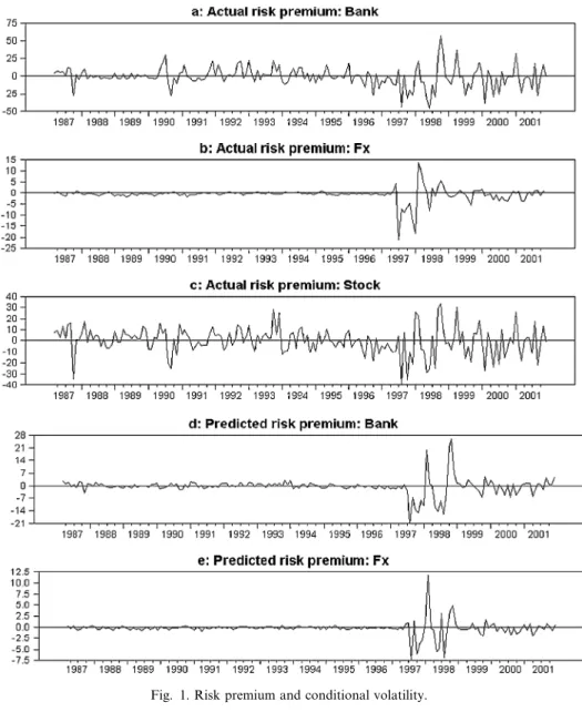
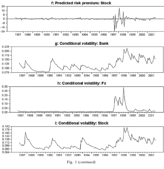
One advantage of modeling the conditional second moments via multivariate GARCH-M approach is that it enables one to recover some interesting statistics such as conditional volatility, and, more importantly, the size of risk premia. These interesting statistics will not be available if one leaves the condition second moments unspecified such as the pricing kernel approach employed by Dumas (1993), Dumas and Solnik (1995), and Tai (1999).11 Table 6 reports those statistics. For example, the predicted monthly risk premium ranges from)0.404% for Bank to 0.337% for
10Engle and Ng (1993) asymmetric tests include the sign bias, the negative size bias, and the positive size bias tests. The sign bias test examines the impact of positive and negative innovations on volatility not predicted by the model. The squared standardized residuals are regressed against a constant and a dummy Stthat takes the value of unity ifet1is negative, and zero otherwise. The test is based on thetstatistic for St. The negative (positive) size bias test examines how well the model captures the impact of large and small negative (positive) innovations, and it is based on the regression of the squared standardized residuals against a constant andStet1ðð1StÞet1Þ. The computedtstatistic forStet1ðð1StÞet1Þis used in this test.
11See the comments provided by Campbell Harvey in Dumas (1993).
World. As for the conditional volatility, it varies between 2.14% for Fx and 11.945%
for Bank. These predicted risk premia and conditional volatilities are both in line with the mean returns and standard deviations of original return series reported in Table 1.
A useful complement to Table 6 is to display the time-series plots of those inter- esting statistics. Fig. 1 contains the plots of actual and predicted risk premia, and conditional volatility for each asset. It can be seen that the dynamics of the predicted risk premia follow very closely to those of actual risk premia, especially during the
Fig. 1. Risk premium and conditional volatility.