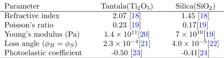
The displacement of the mirrored mechanical oscillator is parametrically coupled to the cavity modea, which has a natural frequency ω0 with y = 0. Hz (thermal noise for the targetφB/φS is indicated in bold and bold numbers should be the minimum in its column); thermal noise spectra for the 38-layer λ/4 stack, provided the measure φB/φS is also listed for comparison.
Laser Interferometer Gravitational-Wave Detectors: An Overview
Gravitational Waves
The remainder of the introductory chapter is devoted to providing some background for Chapters 2, 3 and 4. In a gravitational wave detector, the force Fk acting on the test mass contains a conservative force that provides confinement of the test mass near its zero point. point position as well as an inevitable swinging force.
Laser Interferometry
In this case, we can delve into the detector's local Lorenz frame, in which test masses moving at low velocities are affected by a tidal gravitational field. In this way, the problem of detecting gravitational waves is simplified to measuring a weak classical tidal force field.
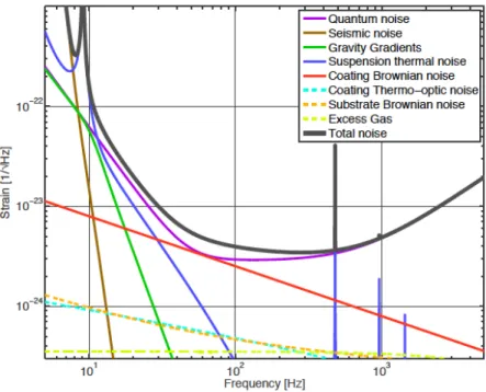
Major Noise Sources of LIGO
This noise arises from thermal fluctuations in the position of the mirror surface sensed by the reflected light - relative to the center of mass of the mirror [10,11]. This is the noisy movement of the center of mass of the test mass driven by thermal fluctuations in the suspension system.
Coating Thermal Noise in Interferometric Gravitational Wave Detectors
Fluctuation Dissipation Theorem
This corresponds to energy loss in the mass and surface of the suspension wire, as well as the attachment points. This refers to the noisy movement of the mirrors driven by ground vibration, after being filtered by the multi-phase seismic isolation system.
Multilayer Dielectric Coatings
Light Beams and Mirror Shapes in Interferometric Gravitational Wave Detectors
Dependence of Thermal Noise on Beam Profile: Scaling Laws
That is, even for p(r) that is non-uniform, we can still consider the wear noise to be inversely proportional to the effective beam area. Scaling laws, strictly speaking, only apply to infinity mirrors with large ray spots and very thin coatings.
Why Modified Beams?
However, for the sizes of test masses and optical beams used in advanced LIGO, Lovelace estimates that the scaling laws cause errors of no more than 15%.
Mode Degeneracy
Quantum Dynamics of Optomechanical Systems
Linear Systems
Most optomechanical systems realized so far operate in the linear regime, in which the linear Heisenberg equations of motion can be written for the mechanical object and the optical field. In case the number of photons inside the cavity is large, we can linearize the annihilation (and creation) operator ˆa for the cavity mode by replacing it with the sum of an averaging term and a perturbation term, then derive a set of linear equations . of movement.
The Simplest Nonlinear Systems
2.2 we express the amplitude and phase of the output field in terms of fluctuations in the coating structure, thereby identifying the various components of the thermal noise of the coating. 2.3 we introduce the loss angles of isotropic coating materials and use the fluctuation-dissipation theorem to calculate the thermal noise cross-spectral density of the coating without considering light penetration into the multilayer coating.
Components of the Coating Thermal Noise
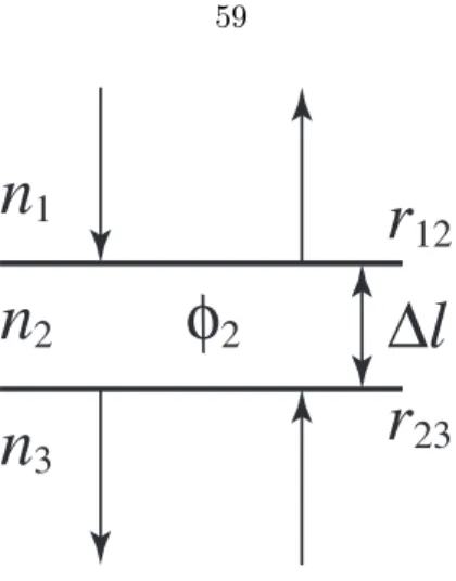
- Complex Reflectivity
- Thermal Phase and Amplitude Noise
- Fluctuations δφ j and δr p
- Mode Selection for Phase Noise
- Conversion of Amplitude Noise into Displacement
Fluctuations in the argument of the complex reflectivity phase modulate the outgoing light and produce direct noise. The first two terms are due to the movement of the coating-air interface at location x and thickness fluctuations of the layers, while the last two terms are due to light penetration into the coating layers.
Thermal Noise Assuming No Light Penetration into the Coating
- The Fluctuation-Dissipation Theorem
- Mechanical Energy Dissipations in Elastic Media
- Thermal Noise of a Mirror Coated with one Thin Layer
- Discussions on the Correlation Structure of Thermal Noise
Using the equation is easy. 2.46) for the calculation of the thermal noise component due to the fluctuation of the position of the coating-air interface - a weighted average [cf. Suppose we would like to measure the weighted average of the mirror surface position, q= ¯ξ=.
Cross Spectra of Thermal Noise Components
- Coating-Thickness Fluctuations
- Fluctuations of Coating-Substrate Interface and Their Correlations with Coat-
- The Anatomy of Coating Thermal Noise
- Full Formula for Thermal Noise
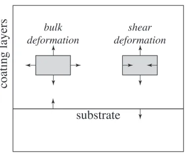
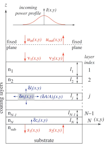
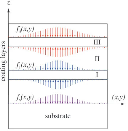
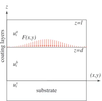
The force distribution pair f1 (f3) in opposite directions acts on opposite sides of layer I (III), while f acts at the coating-substrate interface. To investigate the correlation between the height of the coating-base thickness, zs(~x) and the thickness of each coating layer, δlj(~x), we use a pair of pressures f1(~x) =F0w1(~x ) on the opposite sides of layer I and forcefs(x , y) = F0ws(~x) to the coating-substrate interface (along the -z direction) as shown in Fig.
Effect of Light Penetration into the Coating
Optics of Multilayer Coatings
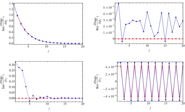
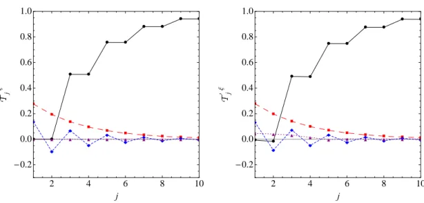
Note that the amount SXj only depends on the material properties (and temperature) of the layer, and is independent of the length of that layer;. the quantities qXj, on the other hand, give us the relative thermal noise contribution of each layer in a dimensionless way. These graphs indicate that for both structures, light penetration is limited within the first 10 layers.
Levels of Light Penetration in advanced LIGO ETM Coatings
We can illustrate the effect of light penetration by showing the relative magnitude of these three contributions for each layer. Note that to focus on the effect of light penetration, we have shown only the first 10 layers.
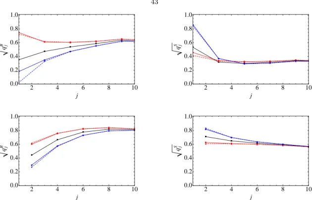
Thermal Noise Contributions from Different Layers
In the figure, the effect of light penetration into the coating layers is embodied in the deviation of the black solid curve from unity in the first few layers, and in the existence of the other curves. We should also expect the effect of photoelasticity (dashed curves) to be small, and the effect of backscattering (giving rise to Tjξc and Tjξs, blue and purple dashed curves) even smaller.
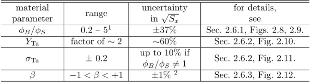
Dependence of Thermal Noise on Material Parameters
- Dependence on Ratios Between Loss Angles
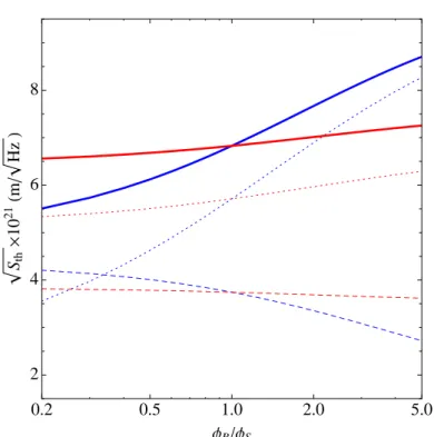
- Dependence on Young’s moduli and Poisson’s ratios
- Dependence on Photoelastic Coefficients
- Optimization of Coating Structure
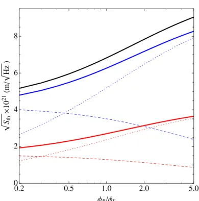
As we vary the ratio between loss angles, there is a moderate change in thermal noise. Hz (the thermal noise for the φB/φS target is given in bold and the numbers in bold should be the minimum within its column); The thermal noise spectra of the 38-layer λ/4 stack assuming the φB/φS target are also listed for comparison.
Measurements of Loss Angles
Bending Modes of a Thin Rectangular Plate
However, in the case where the Poisson's ratio σc of the coating vanishes, the thickness variation depends on the Young's modulus loss angle. The first torsional eigenmodes of such a shell can be used to measure the shear loss angle of the cladding.

Torsional Modes of a Coated Hollow Cylinder
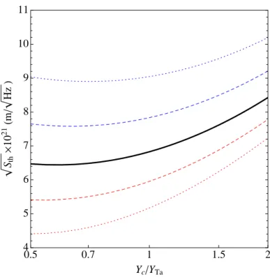
For our baseline parameters, mechanical dissipation is mostly contributed by the tantalum layers, and because the Young's modulus of the tantalum coating material is assumed to be much larger than that of the substrate, the largest contribution to the Brownian noise of the LIGO mirrors is the bending noiseSzszs. By measuring both the thin plate and the cylinder shell, we can obtainφBandφS of the coating.
Conclusions
The φk was intended to characterize the losses incurred by the x-y deformations of the coating, which are measurable when we do not compress the coating, but instead drive the deformations using drum modes of the substrate. 2.6.4 (see Table 2.3) have shown that optimization of the coating structure consistently yields a ∼6% reduction in thermal noise, regardless of φB/φS.
Appendix A: Fluctuations of the Complex Reflectivity due to Refractive index fluc-
- The Photoelastic Effect
- Fluctuations in an Infinitesimally Thin Layer
- The Entire Coating Stack
- Unimportance of Transverse Fluctuations
If the refractive index δn at a particular location δn(z) is driven by the longitudinal strain at that location, the fact that huzz(z0)uzz(z00)i ∝δ(z0−z00) is of concern because it indicates a high variance of δ at any given a single point z with size that is formally infinite, but in reality needs to be described by additional physics (for example, there would be a scale at which the delta function mentioned above starts to resolve). Nevertheless, we find an additional fluctuating contribution to the total complex reflectivity of the multilayer coating.
Appendix B: Elastic Deformations in The Coating
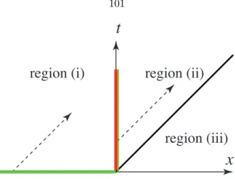
We can thus obtain the stress tensor in the frequency domain for the covering, the nonzero elements for region (a) are given by. Using linear superposition, as well as taking the appropriate limits from the above solution, it is straightforward to obtain elastic deformations in all the configurations required to obtain cross-spectra between different noise.
Appendix C: Definition of loss angle
A reasonable way to define the loss angle is to derive from the fundamental elastic energy equation. Note that the expansion and shear energy UB and US are always positive, so it is consistent to define the loss angle by φB and φS.
Appendix D: Advanced LIGO Style Coating [25]
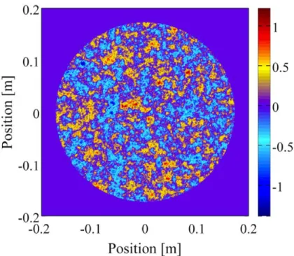
A fundamental limit to the sensitivity of optical interferometers is set by thermal Brownian fluctuations of the mirror surfaces. This thermal noise can be reduced by using larger beams which "average out" the random fluctuations of the surfaces.

Mirror Figure Errors
3.5, we explore two methods to mitigate contrast degradation; neither method was ultimately successful. In this work, we investigate the consequences of realistic mirror errors on the performance of the LG3,3 mode.
Degenerate Perturbation-Theory Analysis
Laugerre-Gauss modes
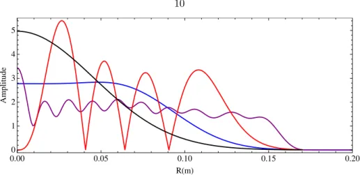
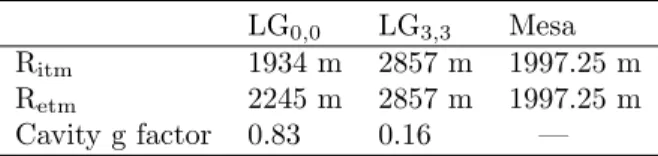
The mode selectivity of the cavity is determined by the finesse of the cavity and the mode-dependent phase shift (2p+|l|+ 1)ψ(z). To allow a fair comparison, the width of all modes considered here and now was chosen to be 0.018 m, which gives a clipping loss [18], due to the finite size of the concave mirrors, of about 1 ppm .
Application of Degenerate Perturbation Theory to the Perturbed Fabry-Perot
- Mode Splitting
- The Modal Input-Output Equation
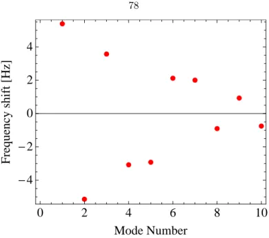
The frequency shift of the degenerate modes introduced by the perturbation is then proportional to the eigenvalues of the matrix. This procedure was applied to the LG3,3 degenerate space using the resonant frequencies from the previous section,ωn.
Contrast Defect
Analytic Calculation
According to Appendix 3.7, the contrast defect in an interferometer with one perfect arm cavity and one disturbed arm cavity can be analytically written as However, depending on the spatial correlations between the mirrors, the contrast defect can be as much as twice the average in some cases.
Numerical Calculation
From these data, the mean and standard deviation of the interferometer contrast error as a function of RMS specular aberration were determined. The simulated contrast error for the Gaussian beam (TEM00) is consistent with the LIGO measured value of around 10-4 [25] and is low enough for efficient detection.
Contrast Defect Improvement
- Better Polishing
- Arm Cavity Detuning
- Mirror Corrections
- Mode Healing
Previous work [27] showed that the presence of a signal recovery cavity can significantly reduce the contrast defect in the case where the resonance mode in the interferometer is TEM0,0. The higher order transverse modes are not resonant in the signal recovery cavity and are therefore suppressed.
Conclusions
In the LG3,3 case, however, the signal cavity is resonant for the LG3,3 mode as well as for all modes that are in the degenerate subspace. In the case where the signal recycling cavity is declared to amplify the gravitational wave response at a certain frequency, the situation could be significantly more complicated due to the frequency splitting shown in Fig. 2b.
Appendix: Contrast Defect
The open quantum dynamics depends on the photon's wave function, whose Fourier transform is related to the photon's frequency content. 4.3, we will give a detailed analysis of the single-photon interferometer, and will calculate the edge visibility of the interferometer; in Sec.
A Single Cavity with one Movable Mirror
- The Hamiltonian
- Structure of the Hilbert Space
- Initial, Final States and Photodetection
- Evolution of the Photon-mirror Quantum State
- Free Evolution
- Junction Condition
- Coupled Evolution
- Full Evolution
Here |ψ1(x, t)im,−∞< x <+∞, is a series of vectors, parameterized byx, in the Hilbert space of the mechanical oscillator, while |ψ2(x, t)i is a single vector in the Space Hilbert of the mechanical oscillator. Equation (4.29) corresponds to the free evolution of the outgoing photon and the mechanical oscillator.
Single-photon Interferometer: Visibility
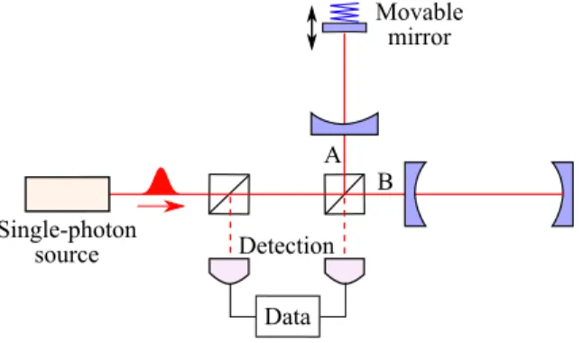
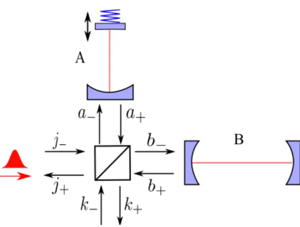
- The Configuration
- Interactions Between Light and Cavities
- The Final State
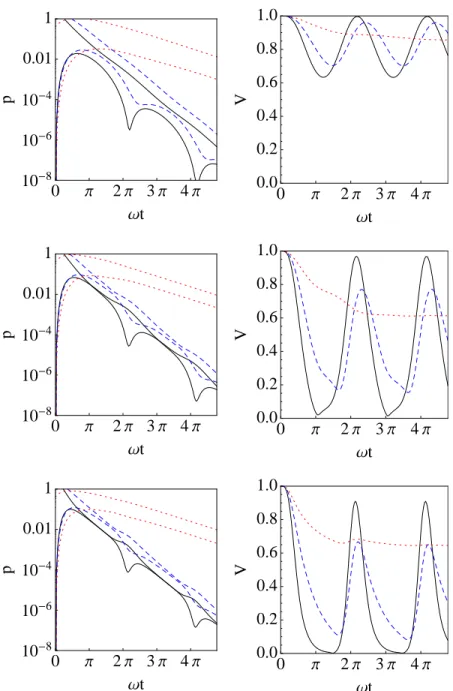
- Examples
For this region we obtain a compact-form solution of . where|φ0i is the initial quantum state of the oscillator, and Mˆ =. the cavity's optical Green function. At any moment, if ψA is proportional to ψB (difference by a phase), the state of the movable mirror does not change, and therefore we have a perfect visibility.
Conditional Quantum-state Preparation
The Configuration
Here, the detuning phase for the mirror on the east arm is adjusted so that the immediately reflected photon will come from the west port, with a probability of 0 coming from the south port. In this case, the appearance of a photon from our detection gate (Fig. 4.6) automatically indicates that the photon has entered the cavity and interacted with the mirror; 4.57) or the conditional quantum state of the mechanical oscillator (non-normalized) is given by:.
Preparation of a Single Displaced-Fock State
Fock modes are simply Fock modes of the oscillator when the photon is inside the cavity, see Eq. This leads to the interesting effect that in the asymptotic limit of τ → +∞ the conditional state will be independent of τ.
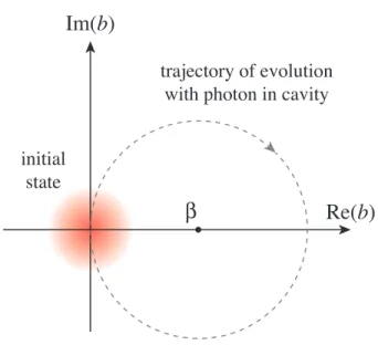
Preparation of an Arbitrary State
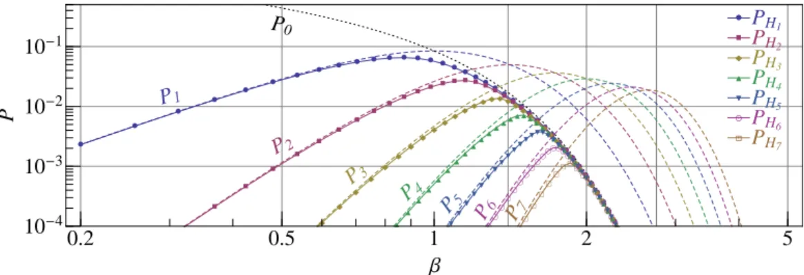
In this frame of reference, the complex amplitude of the coherent modes being superimposed is located on a circle at distance β away from the center, while the target we would like to prepare is simply the Fock mode|ni. To provide a concrete measure of the capability of our state preparation scheme, we have chosen to calculate the minimum probabilities of success for creating all states in the mechanical oscillator's Hilbert subspace spanned by the lowest shifted Fock states, e.g. H1≡Sp {|˜0i,|˜1i},H2≡Sp{|˜0i,|˜1i,|˜2i} etc.
Practical Considerations
Conclusions