Some of these programs are translations of FORTRAN programs that were included in the first and second editions. The name(s) of individual contributors for each program are included in each program.
Television, Radio, Telephone, and Radar Frequency
Antennas
INTRODUCTION
If the peak field strengths of the standing wave are large enough, they can cause arcing inside transmission lines. Standing waves can be reduced and the energy storage capacity of the lines reduced by matching the impedance of the antenna (load) to the characteristic impedance of the lines.
TYPES OF ANTENNAS
- Wire Antennas
- Aperture Antennas
- Microstrip Antennas
- Array Antennas
- Reflector Antennas
- Lens Antennas
These antennas are examined in detail in Chapter 15. c) Microstrip patch array (d) Closed waveguide array Patch. Throughout the book, the radiation characteristics of most of these antennas are discussed in detail.

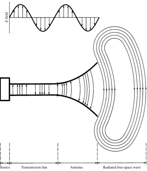
RADIATION MECHANISM
- Single Wire
- Two-Wires
- Dipole
- Computer Animation-Visualization of Radiation Problems
The relative magnitude of the electric field strength is indicated by the density (clustering) of the force lines with arrows indicating the relative direction (positive or negative). Descriptions of the computer programs can be found on the computer disk that accompanies this book.

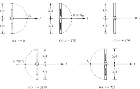
CURRENT DISTRIBUTION ON A THIN WIRE ANTENNA
Ifl < λ, the phase of the current standing wave pattern on each arm is the same throughout its length. Therefore the current in all parts of the dipole does not have the same phase.

HISTORICAL ADVANCEMENT
- Antenna Elements
- Methods of Analysis
- Some Future Challenges
To design antennas with very large directivity, it is usually necessary to increase the electrical size of the antenna. One is the Electric Field Integral Equation (EFIE), and it is based on the boundary condition of the total tangential electric field.
MULTIMEDIA
Umashankar, “FDTD analysis of electromagnetic wave radiation from systems containing antenna horns,” IEEE Trans. Volakis, “Scattering and radiation analysis of three-dimensional arrays of cavities using a hybrid finite element method,” IEEE Trans.
Fundamental Parameters of Antennas
INTRODUCTION
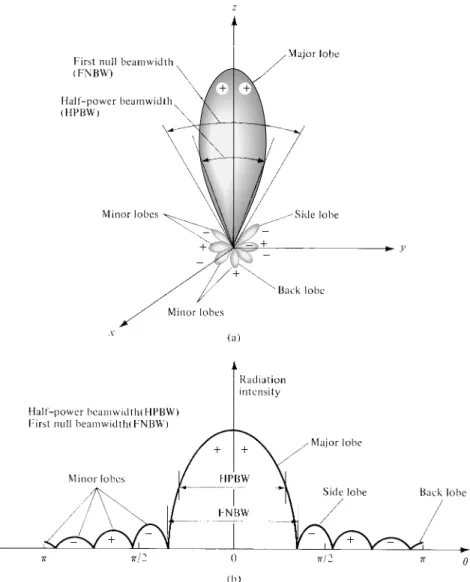
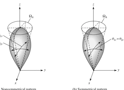
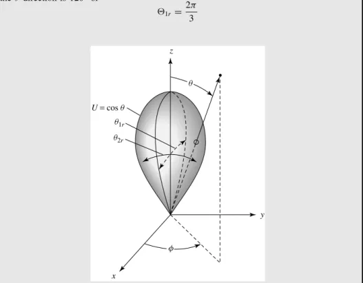
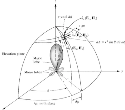
RADIATION PATTERN
- Radiation Pattern Lobes
- Isotropic, Directional, and Omnidirectional Patterns
- Principal Patterns
- Field Regions
- Radian and Steradian
D3/λ from the antenna surface, where λ is the wavelength and D is the largest dimension of the antenna. Far-field (Fraunhofer) region is defined as “that region of the field of an antenna where the angular field distribution is essentially independent of the distance from the antenna.
RADIATION POWER DENSITY
The radial component of the radiated power density of an antenna is given by Wrad=ˆarWr=ˆarA0. To find the total radiated power, the radial component of the power density is integrated over its surface.
RADIATION INTENSITY
E(r, θ, φ)=the antenna's electric field intensity in the far zone =E◦(θ, φ)e−j kr r Eθ, Eφ = the antenna's electric field components in the far zone. For an anisotropic source, U will be independent of the angles θ and φ, as was the case for Wrad.
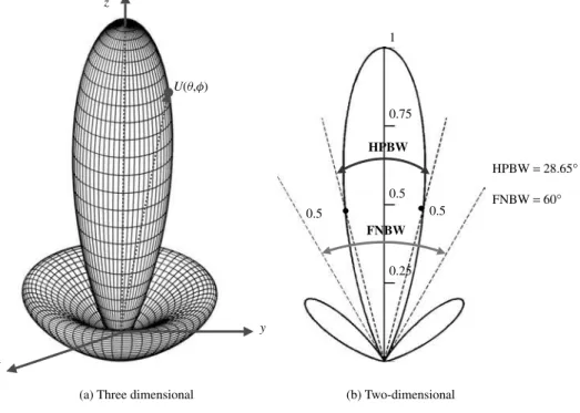
BEAMWIDTH
The most common resolution criterion states that the resolution power of an antenna to distinguish between two sources is equal to half the first zero beamwidth (FNBW/2), which is commonly used to approximate half-power beamwidth (HPBW)[5]. [6]. That is, two sources separated by angular distances equal to or greater than FNBW/2≈HPBW can be resolved from an antenna with a uniform distribution.
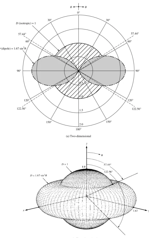
DIRECTIVITY
- Directional Patterns
- Omnidirectional Patterns
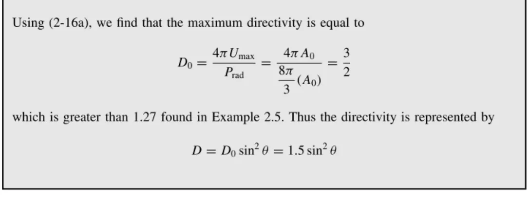
As an illustration, find the maximum directivity of the antenna whose radiation intensity is that of Example 2.2. Determine the maximum directivity of the antenna and express the directivity as a function of the directivity angles θ and φ.
NUMERICAL TECHNIQUES
The value of three more directivity values can also be obtained using Figure 2.18, although they may not be as accurate as those given above because they must be omitted from the graph. Because of the symmetric nature of the function, it can be shown that the shaded area in section #1 (included in the numerical evaluation) is equal to the empty area in section #1 (left out by the numerical method). It should be noted that all functions, although they may contain some symmetry, do not give the same answers regardless of the number of divisions.
ANTENNA EFFICIENCY
In fact, in most cases the answer only approaches the exact value if the number of divisions is increased to a large number. It contains a subroutine that requires the intensity factor U =F (θ, φ) for the required application to be specified by the user. In addition, the upper and lower bounds of θ and φ must be specified for each application of the same pattern.
GAIN
Gain of an antenna (in a given direction) is defined as "the ratio of the intensity in a given direction to the radiation intensity that would be obtained if the power accepted by the antenna were radiated isotropically. The radiation intensity corresponding to the isotropically radiated power is equal to the power accepted (input) by the antenna divided by 4π." Equation form this can be expressed as. It is the loss due to reflection or mismatch loss between the antenna (load) and the transmission line.
BEAM EFFICIENCY
BANDWIDTH
POLARIZATION
- Linear, Circular, and Elliptical Polarizations
- Polarization Loss Factor and Efficiency
The polarization of the wave emitted by the antenna can also be represented on the Poincare sphere [13]–[16]. It is defined, based on the polarization of the antenna in its transmit mode, as. One of the lengths (longer or shorter) will provide right hand (CW) rotation while the other will provide left hand (CCW) rotation.

INPUT IMPEDANCE
W ) (2-85) Of the power supplied by the generator, half is given off as heat in the internal resistance (Rg) of the generator and the other half is delivered to the antenna. If the losses are zero (RL = 0), then half of the trapped power is delivered to the load and the other half is dissipated. Thus half of the power is delivered to the load and the other half is dissipated.
ANTENNA RADIATION EFFICIENCY
This indicates that to supply half the current to the load, you must dissipate the other half. Aperture efficiency (Iap) is defined by (2-100) and is the ratio of the maximum effective area to the physical area. Using (2-86) to (2-89), we conclude that even if aperture efficiencies are higher than 50% (they can be as large as 100%), not all of the power picked up by the antenna is delivered to the load , but it includes what is scattered plus given off as heat by the antenna.
ANTENNA VECTOR EFFECTIVE LENGTH AND EQUIVALENT AREAS An antenna in the receiving mode, whether it is in the form of a wire, horn, aperture,
- Vector Effective Length
- Antenna Equivalent Areas
In general, the total catch area is equal to the sum of the other three, or. For a lossless antenna (RL = 0), the maximum value of the scattering area is also equal to the physical area. If the loss resistance is equal to the radiation resistance (RL= Rr) and the sum of the two is equal to the load resistance (receiver) (RT =Rr+ RL=2Rr), then the effective area is only half of the area. maximum effective area given above.
MAXIMUM DIRECTIVITY AND MAXIMUM EFFECTIVE AREA
If antenna 1 is isotropic, then D0t =1 and its maximum effective area can be expressed as. 2-107) Equation (2-107) states that the maximum effective area of an isotropic source is equal to the ratio of the maximum effective area to the maximum directivity of another source. In general, the maximum effective aperture (Aem) of each antenna is therefore related to the maximum directivity (D0). If reflection and polarization losses are also included, the maximum effective area of (2-111) is represented by.
FRIIS TRANSMISSION EQUATION AND RADAR RANGE EQUATION The analysis and design of radar and communications systems often require the use
- Friis Transmission Equation
- Radar Range Equation
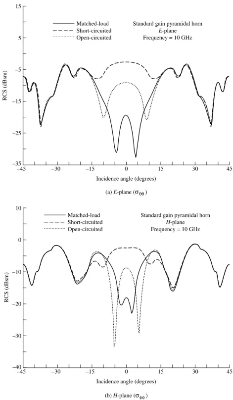
- Antenna Radar Cross Section
Expression (2-124) is used to relate received power to input power, and considers only conduction-dielectric losses (radiation efficiency) of the transmitting and receiving antennas. Relate the shorted, open circuit, and modified RCSs to those of the antenna mode. If the antennas are identical (G0r =G0t =G0) and polarization matched (Pr =Pt =1), the total radar cross-section of the backscatter antenna can be written as.
ANTENNA TEMPERATURE
The temperature appearing at the terminals of an antenna is that given by (2-143) after it is weighted by the gain pattern of the antenna. Assuming no losses or other contributions between the antenna and the receiver, the noise power transmitted to the receiver is given by The results of the above example illustrate that the antenna temperature at the input terminals of the antenna and at the terminals of the receiver can vary by several degrees.
MULTIMEDIA
You must justify (state why?). b) Polarization of the antenna (including axial ratio and sense of rotation, if any). For a frequency of 10 GHz, determine the maximum open circuit voltage at the terminals of the antenna. Assuming that the temperature of the transmission line (waveguide) is 72 ◦F, find the effective temperature at the receiver terminals when the attenuation of the transmission line is 4 dB/100 ft and its length is (a) 2 ft (b) 100 ft.
Radiation Integrals and Auxiliary Potential Functions
- INTRODUCTION
- THE VECTOR POTENTIAL A FOR AN ELECTRIC CURRENT SOURCE J The vector potential A is useful in solving for the EM field generated by a given har-
- THE VECTOR POTENTIAL F FOR A MAGNETIC CURRENT SOURCE M Although magnetic currents appear to be physically unrealizable, equivalent magnetic
- ELECTRIC AND MAGNETIC FIELDS FOR ELECTRIC (J) AND MAGNETIC (M) CURRENT SOURCES
- SOLUTION OF THE INHOMOGENEOUS VECTOR POTENTIAL WAVE EQUATION
- FAR-FIELD RADIATION
- DUALITY THEOREM
- RECIPROCITY AND REACTION THEOREMS
- Reciprocity for Two Antennas
- Reciprocity for Antenna Radiation Patterns
The total fields are then obtained by the superposition of the individual fields due to A and F(John and M). In the previous section we indicated that the solution of the inhomogeneous vector wave equation of (3-14) is (3-27). For reciprocity to hold, it is necessary that the reaction (linking) of one set of resources with the corresponding fields of another set of sources must be equal to the reaction (linking) of the second.

Linear Wire Antennas
INTRODUCTION
INFINITESIMAL DIPOLE
- Radiated Fields
- Power Density and Radiation Resistance
- Radian Distance and Radian Sphere
- Near-Field ( kr 1 ) Region
- Directivity
For a lossless antenna, the real part of the input impedance was referred to as radiation resistance. However, it does contribute to the imaginary (reactive) power which can be used together with the second term of (4-14) to determine the total reactive power of the antenna. The reactive power density, which is most dominant for small values of kr, has both radial and transverse components. For an antenna, the radial sphere represents the volume occupied primarily by the stored energy of the antenna's electric and magnetic fields.

SMALL DIPOLE
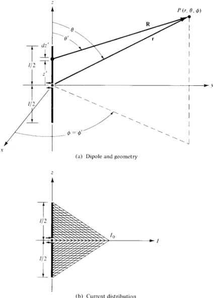
A better approximation of the current distribution of wire antennas, whose length is usually λ/50< l ≤λ/10, is the triangular variant of Figure 1.16(a). The sinusoidal variations of Figures 1.16(b)-(c) are more accurate representations of the current distribution of wire antennas of any length. Since the total length of the dipole is very small (usually l≤λ/10), the values of R for different values of the length of the wire (−l/2≤z≤l/2) do not differ much from r.
REGION SEPARATION
- Far-Field (Fraunhofer) Region
- Radiating Near-Field (Fresnel) Region
- Reactive Near-Field Region
Using this as a criterion, we can write with (4-43) that the maximum phase error must always be. 4-45) Equation (4-45) simply states that to maintain the maximum phase error of an antenna equal to or less than π/8 rad(22.5◦) the sensing distance must be equal to or greater than 2l2/λ where l is the largest∗ dimension of the antenna structure. To find the maximum phase error caused by the omission of the next most significant term, the angle θ at which it occurs must be found. Thus the region where the first three terms of (4-41) are significant, and the omission of the fourth becomes a maximum phase error of π/8 rad (22.5◦), defined by.

FINITE LENGTH DIPOLE
- Current Distribution
- Radiated Fields: Element Factor, Space Factor, and Pattern Multiplication
- Power Density, Radiation Intensity, and Radiation Resistance
- Directivity
- Input Resistance
- Finite Feed Gap
The radiation resistance of a dipole of length l with sinusoidal current distribution, of the form given by (4-56), is expressed by (4-70). To refer to the radiation resistance at the input terminals of the antenna, it is first assumed that the antenna itself is lossless (RL = 0). The values of p become smaller as the wire radius and gap decrease.
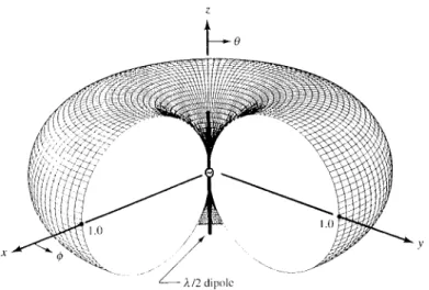
HALF-WAVELENGTH DIPOLE
However, for the l=λ dipole, the current distribution based on (4-56) is quite different, especially at and near the feed point, compared to that based on the moment method, as shown in Figure 8.13(b). This is expected since the current distribution based on the ideal current distribution is zero at the feed point; for practical antennas it is very small. In turn, the values of the input resistance based on the two methods will be quite different, since there is a significant difference in the current between the two methods.
LINEAR ELEMENTS NEAR OR ON INFINITE PERFECT CONDUCTORS Thus far we have considered the radiation characteristics of antennas radiating into an
- Image Theory
- Vertical Electric Dipole
The amount of reflection is generally determined by the respective constitutive parameters of the medium below and above the interface. To excite the polarization of the reflected waves, the apparent source must also be vertical and with polarity in the same direction as the real source (so reflection coefficient +1). Following a procedure similar to the vertical dipole procedure, the virtual source (image) is also placed a distance h below the interface, but with a 180◦ difference in polarity from the real source (thus a reflection coefficient of -1).