The Nutshell Handbook, the Nutshell Handbook logo, and the O'Reilly logo are registered trademarks of O'Reilly Media, Inc. Where these designations appear in this book, and O'Reilly Media, Inc., was aware of a trade-.
Preface
My theory, which is mine
Modeling and approximation
You can review your code and look for optimizations; for example, if you cache previously computed results, you may be able to avoid redundant computation. An advantage of this process is that steps 1 and 2 tend to be quick, so you can explore several alternative models before investing heavily in any of them.
Working with the code
Code style
And finally, one typographical note: throughout the book I use PMF and CDF for the mathematical concept of probability mass function or cumulative distribution function.
Prerequisites
Conventions Used in This Book
Safari® Books Online
How to Contact Us
For more information about our books, courses, conferences and news, please see our website http://www.oreilly.com. Find us on Facebook: http://facebook.com/oreilly Follow us on Twitter: http://twitter.com/oreillymedia Watch us on YouTube: http://www.youtube.com/oreillymedia.
Contributor List
Greg Marra and Matt Aasted helped me clarify the discussion about The Price is Right issue.
Bayes’s Theorem
Conditional probability
Plugging everything into the online calculator at http://hp2010.nhlbihin.net/atpiii/calcu lator.asp, I find that my risk of a heart attack in the next year is about 0.2%, less than the national average. In this example, A represents the prediction that I will have a heart attack in the next year, and B represents the set of conditions I have listed.
Conjoint probability
The usual notation for conditional probability is p A B , which is the probability of A if B is true. Based on an example from http://en.wikipedia.org/wiki/Bayes'_theorem, which no longer exists.
The cookie problem
Bayes’s theorem
I write B1 for the hypothesis that the cookie came from bowl 1 and V for the vanilla cake. The expression on the left is what we want: the probability of dish 1, given that we chose a vanilla cookie.
The diachronic interpretation
There are no other options; at least one of the hypotheses must be true. In the cookie problem there are only two hypotheses – the cookie came from Bowl 1 or Bowl 2 – and they are mutually exclusive and collectively exhaustive.
The M&M problem
In that case we can calculate p D using the law of total probability, which says that if there are two exclusive ways that something can happen, you can add the prob‐ . To get the last column, which contains the posteriors, we divide the third column by the normalizing constant.
The Monty Hall problem
If the car is actually behind door A, Monty can safely open B or C, so he chooses one at random.). And since the car is actually behind A, the chance that the car is not behind B is 1.
Discussion
In this case, the fact that Monty chose B does not reveal any information about the car's location, so it does not matter whether the participant stays or switches. I've included the Monty Hall problem in this chapter because I like it, and because Bayes' theorem makes the complexity of the problem a little more manageable.
Computational Statistics
Distributions
And that would print the frequency of the word 'the' as a fraction of the words in the list. Pmf uses a Python dictionary to store the values and their probabilities, so the values in the Pmf can be any hashable type.
The Bayesian framework
The result is a distribution that contains the posterior probability for each hypothesis, called the (wait for it now) posterior distribution. In the next section, we will solve the Monty Hall problem computationally and then see which parts of the framework are the same.
Encapsulating the framework
In this example, the Likelihood script is a bit complicated, but the Bayesian update framework is simple. Most of the examples in the following chapters follow the same pattern; for each problem we define a new class that extends Suite , inherits Update , and provides Likelihood .
Exercises
If you're familiar with design patterns, you might recognize this as an example of the template method pattern.
Estimation
The dice problem
The most likely alternative is the 6-sided die, but there is still almost a 12% chance of 20s. Now the probability is 94% that we roll the 8-sided deck and less than 1% for the 20-sided deck.
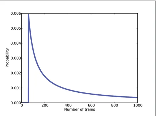
The locomotive problem
Otherwise, the question is, "Given that there are hypo sides, what is the chance of rolling data?" The answer is 1/hypo regardless of data. For any given value of N, what is the probability of seeing the data (a locomotive with number 60).
What about that prior?
The mean of the posterior is 333, so this can be a good guess if you want to minimize error. If you played this guessing game over and over again, the mean of the posterior would be reduced to the mean square error of your estimate over the long run (see http:// . en.wikipedia.org/wiki/Minimum_mean_square_error).
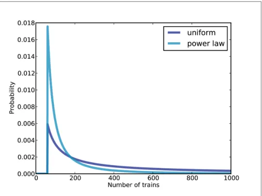
An alternative prior
Using the basic information represented in the power law prior, we can eliminate values of N greater than 700. So the power law prior is more realistic because it is based on general information about the size of companies and behaves better in practice.
Credible intervals
A simple way to calculate a credible interval is to sum the probabilities in the posterior distribution and record the values corresponding to the 5% and 95% probabilities. For the previous example—the locomotive problem with a forward power law and three trains—the 90% credible interval is 91,243.
Cumulative distribution functions
The German tank problem
But if, as with the locomotive problem, you don't have much data, use relevant backup. As an exercise, implement the probability function for this variation of the locomotive problem and compare the results.
More Estimation
The Euro problem
The likelihood function is relatively easy: If Hx is true, the probability of heads is x/100 and the probability of tails is 1−x/100.
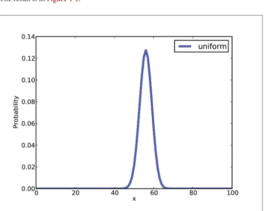
Summarizing the posterior
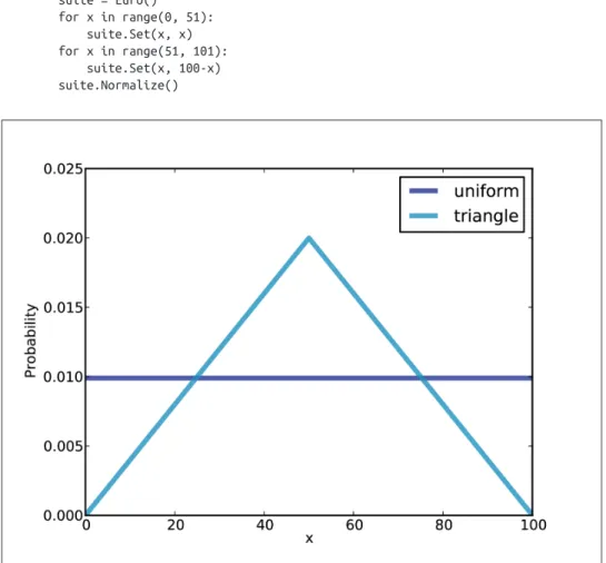
Swamping the priors
It may be more reasonable to choose a prior that gives a higher probability to values of x near 50% and a lower probability to extreme values. This is an example of transferring the priors: with enough data, people starting with different priors will tend to converge on the same posterior.
Optimization
We can speed things up even more by rewriting Likelihood to process the entire dataset instead of one spin at a time. As an alternative, we could encode the data set as a tuple of two integers: the number of heads and tails.
The beta distribution
The shape of the beta distribution depends on two parameters, written α and β, or alpha and beta. So that's great, but it only works if we can find a beta distribution that's a good choice for a previous one.
Odds and Addends
Odds
The odds form of Bayes’s theorem
If the odds are 5:1 against my horse, then five out of six people think she will lose, so the probability of winning is 1/6.
Oliver’s blood
If Oliver is one of the people who left blood at the crime scene, then he is responsible for the 'O' sample, so the probability of the data is just the probability that a random member of the population has type 'AB' . The probability of the data is slightly higher if Oliver is not one of the people who left blood at the scene, so the blood data is actually evidence against Oliver's guilt.
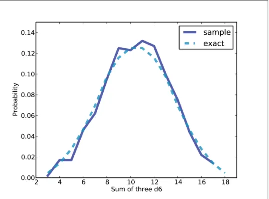
Addends
This example is a bit contrived, but it is an example of the counterintuitive result that data consistent with a hypothesis is not necessarily in favor of the hypothesis. Given two Pmfs, you can enumerate all possible pairs of values and calculate the distribution of the sums.
Maxima
So to find the distribution of the maximum of k values, we can enumerate the proba‐. The running time of this method is proportional to m, the number of elements in the Cdf.
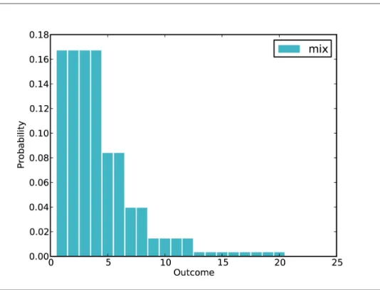
Mixtures
In general, we need to know the probability of each die in order to weight the results appropriately. Values above 12 are unlikely because there is only one die in the box that can produce them (and it does so less than half the time).
Decision Analysis
The Price is Right problem
The code I wrote for this chapter is available at http://think bayes.com/price.py; reads data files that can be downloaded from http://thinkbayes.com/.
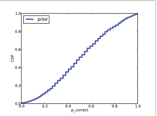
The prior
Probability density functions
Representing PDFs
Pdf provides an implementation of MakePmf, but not Density, which must be provided by an underlying class. In that case, we can use a sample to estimate the PDF of the entire population.
Modeling the contestants
Can we calculate a likelihood function; that is, for each hypothetical price value, can we calculate the conditional probability of the data. According to this model, the question we need to answer is: "If the current price is the price, what is the probability that the competitor's valuation is assumed?".
Likelihood
Update
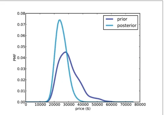
PmfPrice generates a discrete PDF approximation of the price that we use to construct the prior. The posterior is shifted to the left because your guess is at the lower end of the previous range.
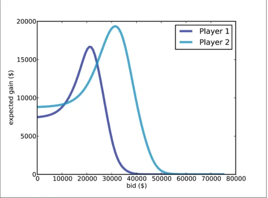
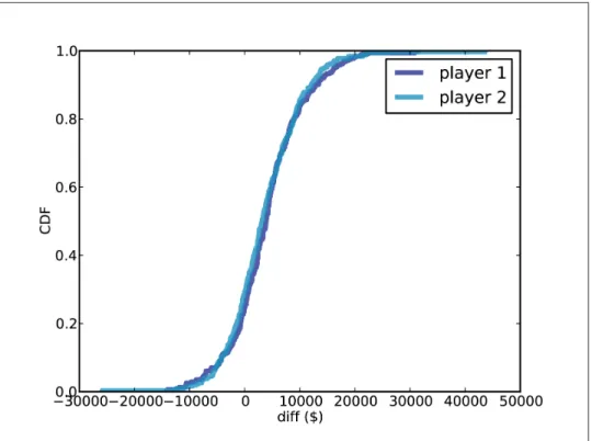
Optimal bidding
ExpectedGain loops through the values in the posterior and calculates the gain for each bid, given the actual prices at the showcase. One of the characteristics of Bayesian estimation is that the result comes in the form of a posterior distribution.
Prediction
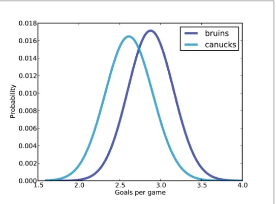
The Boston Bruins problem
Again, we use numpy.linspace to make an array of n equally spaced values between low and high, including both. So the prior distribution is Gaussian with mean 2.7, standard deviation 0.3, and it spans 4 sigmas above and below the mean.
Poisson processes
Returning to the hockey problem, here is the definition for a set of hypotheses about the value of λ. The benefit of using this model is that we can calculate the distribution of goals per game efficiently as well as the distribution of time between goals.
The posteriors
Customers are more likely to go to a store at certain times of the day, buses are supposed to arrive at fixed intervals, and goals are more or less likely at different times during a match.
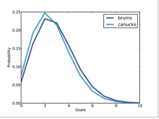
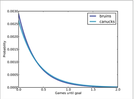
The distribution of goals
So the overall distribution of measures is a mixture of these Poisson distributions, weighted by the probability in the distribution of lambs. For each value of lamb, we create a Poisson Pmf and add it to the meta-Pmf.
The probability of winning
Sudden death
In the event of a tie at the end of "regulation play", the teams play overtime periods until one team scores. Thanks to Dirk Hoag at http://forechecker.blog spot.com/, I was able to get the number of goals scored during regulation (not overtime) play for each game in the regular season.
Observer Bias
The Red Line problem
The model
If you stood on the platform from The average time between trains, as seen by a random passenger, is significantly higher than the true average.
Wait times
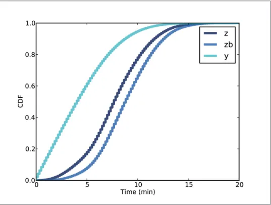
So given the actual distribution of the holes we can calculate the distribution of the holes as seen by passengers. To see why, remember that for a given value of zp, the distribution of y is uniform from 0 to zp.
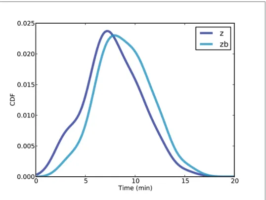
Predicting wait times
The posterior distribution of x shows that, after seeing 15 passengers on the platform, we believe that the time since the last train is probably 5-10 minutes. The predictive distribution of y indicates that we expect the next train in less than 5 minutes, with about 80% confidence.
Estimating the arrival rate
The data is a pair, y, k, where y is a waiting time and k is the number of passengers who arrived. But in both cases the likelihood is the probability of seeing k arrivals in a time period, given lam.
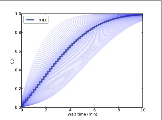
Incorporating uncertainty
But the spread of the posterior distribution captures our uncertainty about λ based on a small sample. Perform the analysis for each parameter value and generate a set of predictive distributions.
Decision analysis
We can do this by extending the distribution of lam to include large random values. Finally, we can calculate the inverse of BiasPmf to obtain from the distribution of zb in distri‐.
Two Dimensions
Paintball
The suite
Given a floor plan of the room, we might be able to choose a more detailed prior, but we'll start simple.
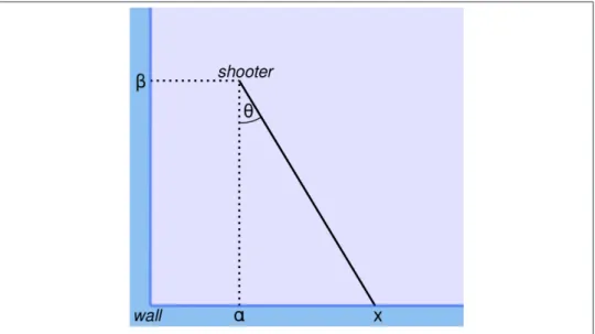
Trigonometry
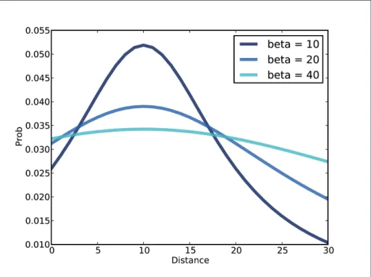
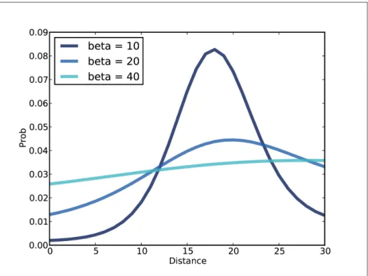
For all values of beta, the most likely splash location is x = 10; as beta increases, so does the spread of Pmf. We can use MakeLocationPmf to calculate the probability of any value of x, given the opponent's coordinates.
Joint distributions
Again, alpha and beta are the hypothetical coordinates of the shooter, and x is the location of an observed splash. So the data provides evidence that the shooter is on the near side of the room.
Conditional distributions
The result is the distribution of the ith variable under the condition that the jth variable is val. The distribution of one parameter in a joint distribution depending on one or more of the other parameters.
Approximate Bayesian Computation
The Variability Hypothesis
And answering this question gives me a chance to demonstrate some techniques for working with large data sets. We'll start with the simplest implementation, but it only works for datasets smaller than 1000 values.
Mean and standard deviation
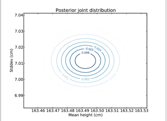
If the true parameters of the distribution are μ and σ and a sample of n values is taken, then the estimator of μ is the sample mean, m. This process may seem bogus because we use the data to select the range of the previous distribution and then use the data again to update.
The posterior distribution of CV
We use the data to select the range for the prior, but only to avoid calculating many probabilities that would have been very small anyway. With num_stderrs=4, the range is large enough to cover all values with a non-negligible probability.
Underflow
Before applying the log transformation, Log uses MaxLike to find m, the highest probability in Pmf. Using log-likelihoods avoids the problem of underflow, but while Pmf is under the log transformation, there is not much we can do about it.
Log-likelihood
A little optimization
For example, in the euro problem, we don't care about the order of coin flips, only the total number of heads and tails. We can use these sampling distributions to calculate the probabilities of the sample statistics, m and s, given hypothetical values for μ and σ.
Robust estimation
We can convert from ipr to an estimate of sigma using the Gaussian CDF to calculate the portion of the distribution covered by a given number of standard deviations. For example, it is a well-known rule of thumb that 68% of a Gaussian distribution falls within one standard deviation of the mean, leaving 16% in each tail.
Who is more variable?
So another interpretation of ABC is that it represents an alternative model of like. When we calculate p DH , we ask "What is the probability of data under a given hypothesis?".
Hypothesis Testing
Back to the Euro problem
In that case we would say that "one-sided" means that the probability of heads is 140/250. So we would say that the data is evidence in favor of this version of B.
Making a fair comparison
It is not clear how to calculate the probability of B, because it is not clear what. To calculate the probability of b_uniform, we calculate the probability of each subhypothesis and collect a weighted average.
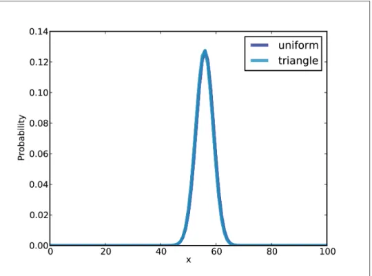
The triangle prior
The likelihood ratio for b_uniform is 0.47, which means the data is weak evidence against b_uniform, compared to F. The likelihood ratio for b_triangle is 0.84, compared to F, so again we would say the data is weak evidence against B.
Evidence
Interpreting SAT scores
The scale
To keep things simple, I interpret the raw score as the number of correct answers, for example. With this simplification, the probability is given by the binomial distribution, which calculates the probability of k correct answers from n questions.
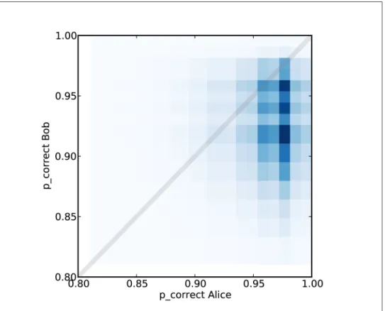
Posterior
To calculate the likelihood of A, we can count all pairs of values from the posterior distributions and add up the total probability of cases where p_correct is higher for Alice than for Bob. If we use more values, c_like is smaller, and at the extreme, if p_correct is continuous, c_like is zero.
A better model
Given the distribution of efficiency across test takers and the distribution of difficulty across questions, we can calculate the expected distribution of raw scores. MakeRawScoreDist takes efficiency, which is a Pmf representing the distribution of efficiency across test subjects.
Calibration
Someone with an efficiency of 3 (two standard deviations above the mean) has a 99% chance of answering the easiest questions on the exam and a 78% chance of answering the hardest. At the other end of the range, someone who is two standard deviations below the mean has only a 24% chance of answering the easiest questions.
Posterior distribution of efficacy
Again we use TopLevel and compare A, the hypothesis that Alice's efficacy is higher, and B, the hypothesis that Bob's is higher. If we rather believe that A and B are equally likely, then in light of this evidence we would give A a posterior probability of 77%, leaving a 23% chance that Bob's efficacy is higher.
Predictive distribution
We compare the two predictive distributions to calculate the probability that Alice will receive a higher score again. The posterior probability is 3:1 that Alice's efficacy is higher, but only 2:1 that Alice will do better on the next exam.
Simulation
The Kidney Tumor problem
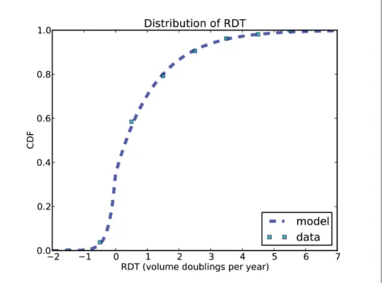
Nevertheless, I was able to extract the data I needed by printing one of their graphs and measuring it with a ruler. The squares are the data points from the paper; the line is a model I fit to the data.
A simple model
According to the data of Zhang et al., only 20% of tumors grew so rapidly during an observation period. So again, I concluded that it was “more likely than not” that the tumor had formed before the date of discharge.
A more general model
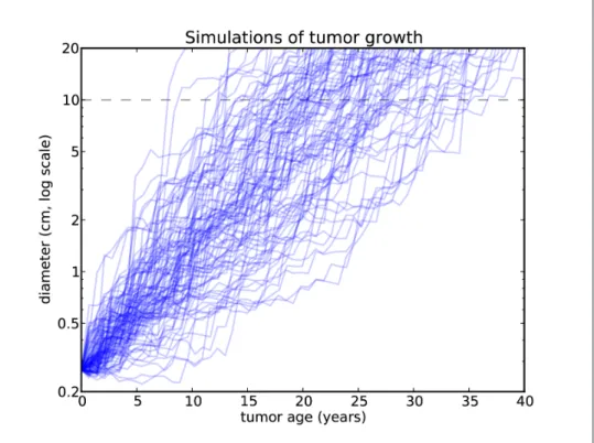
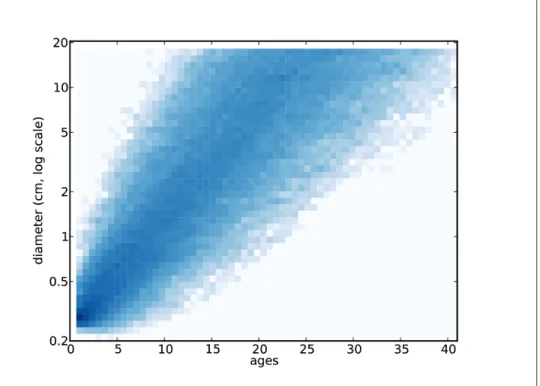
In the data source, the range of observed sizes is from 1.0 to 12.0 cm, so we extrapolate beyond the observed range at each end, but not far and not in a way that is likely to significantly affect the results. To convert from one to the other, I again use the volume of a sphere with a given diameter.
Implementation
Caching the joint distribution
By taking a vertical section of the joint distribution, we can obtain the distribution of sizes for a given age. Here is the code that reads the joint distribution and constructs the conditional distribution for a given size.
Serial Correlation
So if there is a relationship, it's likely to be weak, at least in this size range. The difference is modest for low percentiles, but for the 95th percentile it is more than 6 years.
A Hierarchical Model
The Geiger counter problem
Now we want to go the other way: given the data, we want the distribution of pa‐. And if you can solve the forward problem, you can use Bayesian methods to solve the inverse problem.
Start simple
Make it hierarchical
Each hypothesis is a detector, so we can call SuiteLikelihood to get the probability of the data under the hypothesis. So instead of updating the transmitter and then the detectors, we can do both steps at the same time, using the result from Detector.Update as the probability of the transmitter.
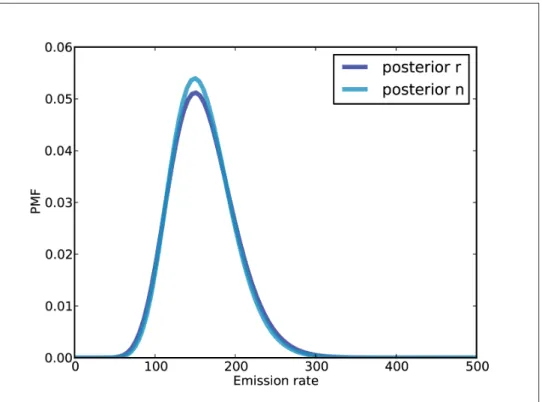
Extracting the posteriors
For each value of r, we have a range of values for n, and the prior distribution of n depends on r. We calculate a posterior distribution of n for each value of r, then we calculate the posterior distribution of r.
Dealing with Dimensions
Belly button bacteria
Lions and tigers and bears
Here the data is a sequence of counts in the same order as the parameters, so in this case it should be the number of lions, tigers and bears. Here is the code that updates the dirichlet with the observed data and calculates the posterior marginal distributions.
The hierarchical version
Because Dirichlet.Likelihood does not actually calculate the probability of the data under the entire Dirichlet distribution. The first term, cx, is the multinomial coefficient; I leave it out of the calculation because it is a multipli‐.
Random sampling
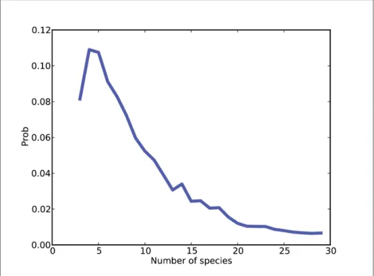
If we have background information on the number of species in the environment, we can choose a difference. If you're not interested in the details, feel free to skip to "The Umbilical Data" on page 175, where we look at results from the umbilical data.
Collapsing the hierarchy
If the number of species is large, the probability of the data may be too small for floating point data (see “Undercurrent” on page 109). For each value of n, we must divide the row by the total of the first n values of gamma.
One more problem
This correction is necessary because every time we see a species for the first time, we have to consider that there were a number of other unseen species that we may have seen. For larger values of n, there are more invisible species that we could have seen, increasing the likelihood of the data.
We’re not done yet
We need to use a correction factor for the number of unseen species, as in Spe cies4.Likelihood. The difference here is that by multiplying the set, we update all the probabilities at once.
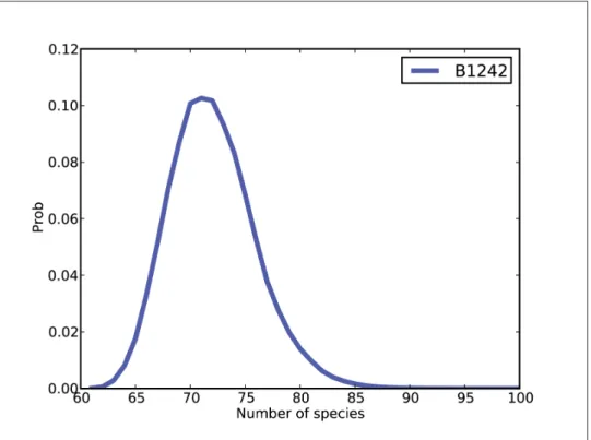
The belly button data
There are a few dominant species that make up a large proportion of the total, but many species that yielded only a single reading. The most common species accounts for 23% of the 400 reads, but since there are almost certainly unseen species, the most likely estimate for its prevalence is 20%, with a 90% credible interval between 17% and 23%.
Predictive distributions
Each time through the loop we add a new observation to the seen and record the number of reads and the number of new species so far. The result of RunSimulation is a dilution curve, represented as a list of pairs with the number of reads and the number of new species.
Joint posterior