Complex amplitudes of force ratio and moment ratio on smooth rigid wall for harmonic forcing. Complex amplitude of force ratio and moment ratio on smooth rigid wall for harmonic forcing.
INTRODUCTION
WALL TYPES
A wide variety of types of soil retaining wall structures are used in civil engineering works. Some of the more common types of wall structures are shown schematically in Fig.
TYPE I TYPE Il
WALL TYPES
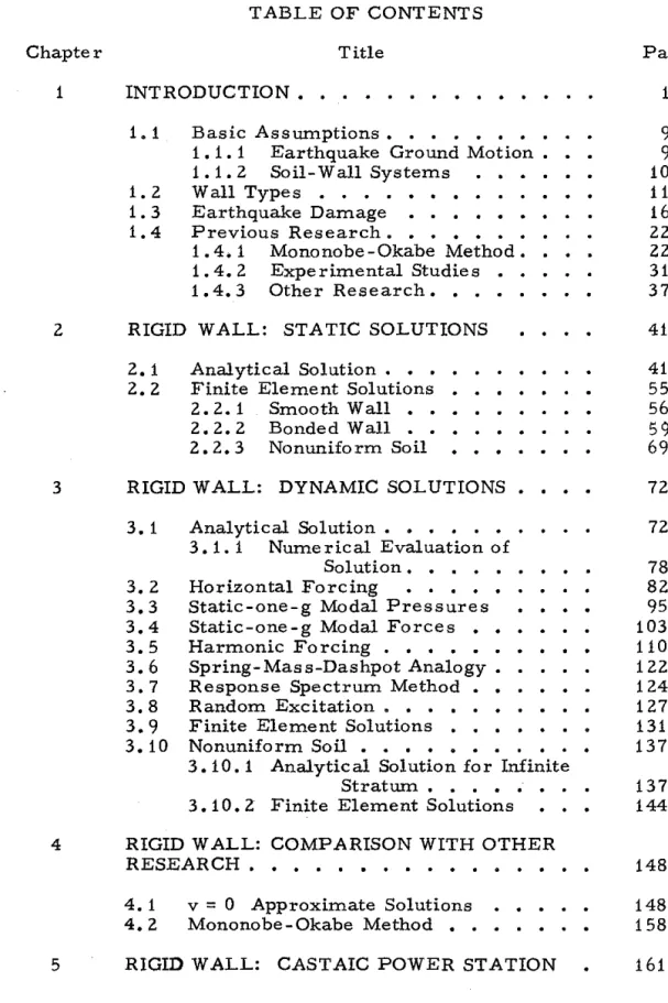
EARTHQUAKE DAMAGE
Details of the reservoir and the damage are given by Housner, Jennings and Brady in Reference (21). The damaged sections of the Wilson Canyon Canal were near Olive View Hospital.
PREVIOUS RESEARCH
Okabe value would be expected when the outward movement of the top of the wall was less than about O. 5 inches. Details of the Mononobe-Okabe method and suggestions regarding its application to design problems are given by Seed and Whitman(SO).
MONONOBE-OKABE ANALYSIS
Also, in the Mononobe-Okabe method, it is usual to neglect the influence of the dynamic behavior of the structure on the pressures. Details of the model used for the rigid wall problem are shown in Fig.
SCOTT'S MODEL
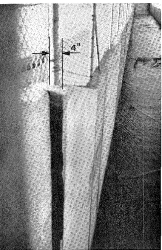
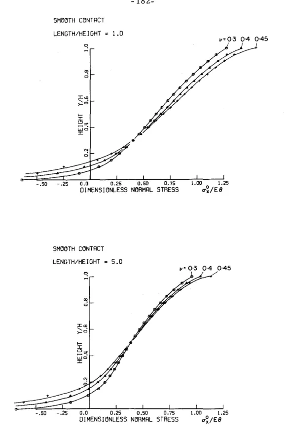
The vertical end boundaries are taken to represent rigid walls, and the contact between the homogeneous linearly elastic soil and the wall is assumed to be smooth; that is, the vertical boundaries are assumed to be free of shear stresses. For simplicity, the magnitude of this body force is taken as '{, the unit weight of the earth, and thus represents the application of a static horizontal acceleration of a g.
RIGID WALL PROBLEM
FINITE ELEMENT SOLUTIONS
A comparison was made between the analytical solution of the previous section and a solution of the same problem calculated by the finite element method. The antisymmetry of the problem was used to halve the mesh length. In view of the excellent results obtained by the finite element method for the smooth rigid wall problem, it appears.
The exact nature of the stress distribution at the wall boundary for the vertical gravity load case is difficult to calculate because the stresses depend on the way in which the soil is placed behind the wall during construction. In cohesionless soil, the absence of significant confining stresses near the top of the wall will cause yielding at very low stress levels. In this case, the normal pressure at the top of the wall will be essentially zero, regardless of the boundary conditions at the wall.
Assuming the Mohr-Coulomb failure criterion, it is easy to prove that the limiting pressure on the wall is given by. It can be seen that the failure of cohesionless soil significantly reduces the elastic pressure distributions in the range fr> O.
To show the influence of nonlinear soil behavior on the stress singularity, a finite element analysis for the bonded-contact rigid wall was performed using the bilinear material properties shown in Fig. 2 =principal stresses in the x-y plane The mesh and the elements described for the previous bonded contact solutions were used again. It can be seen that the overall effect of the nonlinear behavior on the wall pressure distribution is not very pronounced.
The stresses in the top three elements are reduced by the layer, but this reduction is offset by an increase in the stresses below the yield zone. In the following section, the influence of a variation of the elastic constants with depth is studied, and that is.
RIGID WALL: DYNAMIC SOLUTIONS 1. ANALYTICAL SOLUTION
For non-trivial solutions of equations (3.6), the determinant of the coefficients of C and D must vanish. There is a degenerate form of the solution in which the displacements are constant with respect to the x-direction. It is also convenient to express the solutions in terms of the following dimensionless parameters.
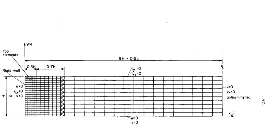
Thus the normal pressure distribution on the wall, resulting from an arbitrarily rigid time horizontal acceleration. It is informative to show the relationship between this representation of the static solution and the forced dynamic solution. The dimensionless natural frequencies, static-one-g modal forces, and moments for the plotted pressure distributions and for some of the higher mode distributions are given.
In general, the plot shows only the modal force values that exceed 5% of the static wall force for n = 1 cases. 17 shows the variation in the location of the pressure centers of the modal pressure distributions and can be used to calculate the static et-g modal moments.
RANDOM EXCITATION
Statistical estimates of seismic wall forces and moments can be calculated from earthquake power spectral density and steady-state solutions for harmonic forcing using some basic results of random vibration theory. If we assume a zero mean for the earthquake input and express (3.48) in terms of the parameters of the wall problem, we get Statistical estimates of the maximum forces and moments can be found from the root mean square responses using the properties of the normal distribution curve.
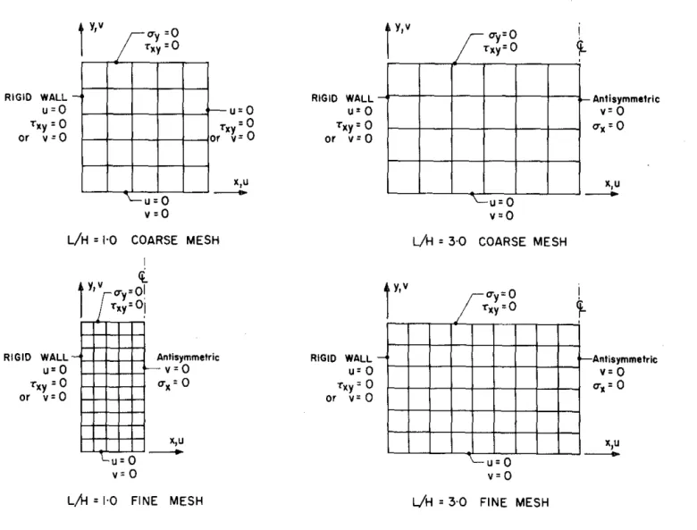
Details of the use of this method for evaluating the response of buildings to earthquakes are given by Tajimi (54l. The finite element method has been used to calculate the normal modes of solutions for a number of rigid wall problems. The purpose of this study was to verify the accuracy of the finite element method for this type of problem with comparison with the analytical solution for a smooth wall and to investigate the effect of the wall-soil contact assumption on the dynamic behavior.the antisymmetric modes below are compared in Tables and 3.4 below.
0 coarse and fine meshes were used in the static finite element analysis for the horizontal body force and produced pressure distributions within 10% and 7% of the static analysis results, respectively. A fairly good agreement can be observed between the equivalent frequencies and modal pressure distributions of the smooth and bonded contact cases.
NONUNIFORM SOIL
The analytical and fine-mesh finite element results for both frequencies and pressure distributions show agreement within 5%. From these solutions it appears that satisfactory results can be obtained for modes having at least four elements within the modal wavelength. It is therefore unlikely that the wall-soil interface condition will have a significant influence on the earthquake-induced pressures.
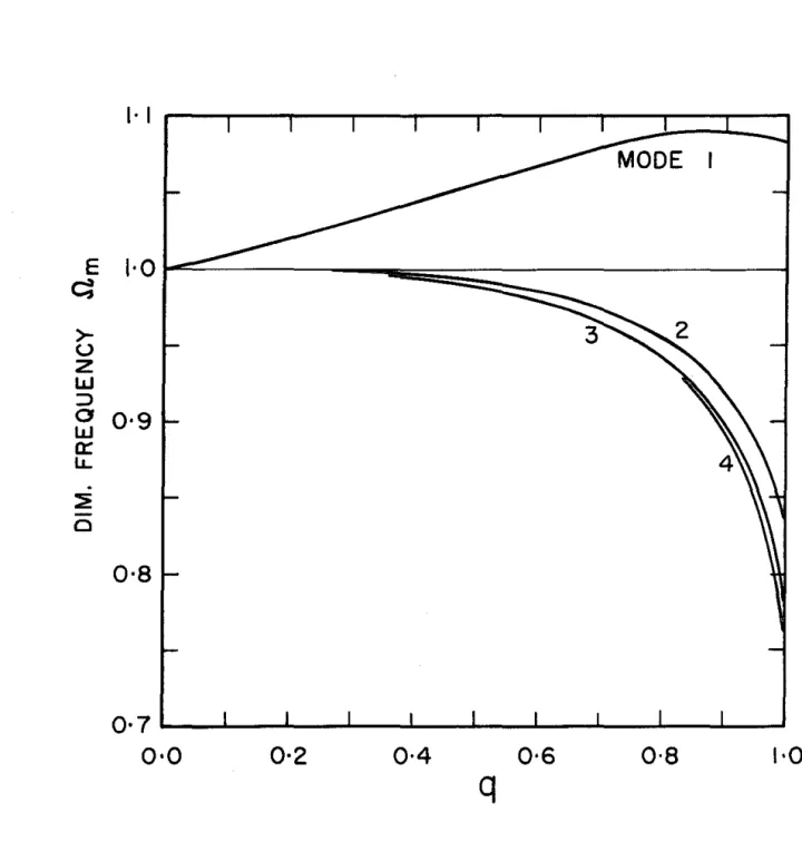
2, 3.3 and 3, 4 it can be seen that for ~ values greater than 5 all n = 1 modes have frequencies within 25% of the infinite pure horizontal shear and vertical dilitation frequencies of the layer. Hence the natural frequencies of the A non-uniform infinite layer can be expected to be reasonably good approximations to the frequencies of the low n-modes of the non-uniform bounded problem with relatively large values. In view of this approach, it was considered informative to present the frequency solution for an. Under the assumption of plane strain and no variation in the x-direction of the displacements, substituting the stress-strain relations into the equilibrium equations yields the equations of motion as. These equations are decoupled and it is clear that the solution of the second equation can be obtained directly from the first.
NONUNIFORM STRATUM
BYj_ (~~)
- RIGID WALL: COMPARISON WITH OTHER RESEARCH
- RIGID WALL: CASTAIC POWER STATION
The dimensionless natural frequencies of the lowest four modes are plotted as a function of the parameter q in the figure. The natural frequencies of the six lowest antisymmetric modes (in the order given by the finite element analyses) are given in Tables 3. The modal pressure of the static single g distribution evaluated from expression (4.7) is compared with some exact examples of smooth walls in Fig.
Typical equations of the v = 0 and the exact amplitudes of the wall force with smooth wall complexes are shown in Figure. The equation given here is made based on the solutions of the static-elastic theory. 3 shows details of the structure and the soil placed along the building during construction.
In the application of the analytical solution, the soil body was represented by an equivalent rectangle with ~ = 1. The natural frequencies of the modes that made a significant contribution to the wall pressure distributions are given in Table 5.1.
CASTIC PROBLEM
MESH FOR NORMAL MODES
FORCED WALL
- STATIC ANALYTICAL SOLUTION
It is convenient to evaluate the earthquake-induced pressures on deformable wall structures by obtaining the solution in two parts. If the wall-soil system is assumed to be linear, the principle of superposition can be used to combine these two solutions to obtain the total stresses induced by the earthquake. To obtain a substantially accurate solution, a superposition in the frequency domain must be performed using the harmonically forced steady-state solutions for both cases.
In this chapter, the solutions for the static and harmonic displacement at the wall boundary are presented. In Chapter 7, these solutions are superimposed on the rigid wall solutions to give the total earthquake forces and moments on the deformable wall. It is clear that it is not possible to consider all types of wall deformations in a general study, and in this study only a rotational deformation of the wall around its base is considered in detail.
The methods used for rotational deformation can be extended to analyze other forms of wall displacement. An analytical solution is presented in this section for the pressures on a smooth wall resulting from a static rotational displacement.
DISPLACEMENT FORCING OF WALL
By substitution, we can show that the general form of the solution of the equations is (6. 6). For the special case n = 0, the partial differential equations reduce to a single equation given by It appears that the Fourier integral of the formal solution cannot be expressed in analytical form; however, we can use approximate expressions and numerical methods to provide solutions.
Solutions to forcing from a higher-order displacement function at the wall boundary can be evaluated by assuming a solution of the form The pressures on the statically rotated wall of the problem shown in Fig. 6.1 and studied in the previous section were evaluated using the finite element method. The forces and moments of the wall (about the base of the wall) were calculated by numerical integration of the finite element pressure distributions and are shown in Fig.
The wall pressure, forces and moments are dependent on the earth's moduli of elasticity (E or G) and the magnitude of the rotation 9. Consequently, these variables appear in the dimensionless parameters used in the pressure and force plots. Except for the region at the top of the wall (g > O. 8), where the bound wall stresses become singular, the agreement between the smooth and bound pressure distributions is moderately good.
SMCJCJTH CCJNTRCT
DIMENSICJNLESS NCJRMRL STRESS ~~/EB


