Are All Central Bank Interventions Created Equal? An Empirical Investigation

Are all Central Bank interventions created equal? An empirical investigation

Stephen Sapp

Richard Ivey School of Business, University of Western Ontario, London, Ont. N6A 3K7, Canada Received 8 November 2001;accepted 14 August 2002

Abstract

This study investigates the relationship between Central Bank interventions and technical trading rule profitability in the spot foreign exchange market. Because interventions are not necessarily exogenous events, we analyze the relationships between interventions by the G-3 Central Banks, financial market conditions, changes in monetary policy and technical trading profitability. By considering announced, unannounced, unilateral and coordinated interven- tions separately, we provide more insight into the interrelationships between these factors than previous studies. We find that the level of technical trading profits and market uncertainty in- crease preceding and remain high during interventions, especially announced and coordinated, but decrease afterward. A preliminary investigation of the possible role of a time-varying risk premium around interventions cannot be rejected.

Ó 2003 Elsevier B.V. All rights reserved.

JEL classification:F31;G14;E58

Keywords:Foreign exchange;Central Bank intervention;Technical analysis

1. Introduction

Because the foreign exchange market is the largest and arguably most important financial market in the world, it is believed that if any financial market should be efficient it should be this market. Unfortunately tests of even the weakest form of market efficiency are rejected in the foreign exchange market – technical analysis is consistently profitable. This apparent inefficiency has persisted from the first studies (Poole, 1967;Dooley and Shafer, 1976, 1983) to the most recent studies

www.elsevier.com/locate/econbase

E-mail address:ssapp@ivey.uwo.ca(S. Sapp).

0378-4266/$ - see front matter Ó 2003 Elsevier B.V. All rights reserved.

doi:10.1016/S0378-4266(02)00410-7

(Neely et al., 1997;Gencßay, 1999;LeBaron, 1999;Neely, 2002). Researchers have proposed that Central Banks may play a role in this apparent inefficiency because they can influence the supply and demand for currencies at any time. Consequently exchange rates are not always determined by the laws of supply and demand re- quired for market efficiency (Friedman, 1953;Dooley and Shafer, 1983;Corrado and Taylor, 1986;Sweeney, 1986 among others).

Consistent with the hypothesis that Central Banks may be related to this apparent inefficiency, Szakmary and Mathur (1997), Neely (1998) and LeBaron (1999) find that technical trading profits were correlated with periods of Federal Reserve inter- vention activity during the 1980s and early 1990s. To better understand this relation- ship Neely (2002) uses higher frequency data and finds that the profitability of technical analysis actually begins before the start of intervention activities. We build on these studies by investigating differences across types of interventions (e.g. an- nounced versus unannounced) and whether interventions and these periods of appar- ent inefficiency may be related to some other economic factor(s).

We address these issues using a dataset that is longer and more comprehensive than those used in previous studies. We have both a period of extensive intervention activ- ity (the 1980s and early 1990s) as well as a period with little intervention activity (the mid- to late-1990s). This permits us to compare different types of interventions by the Federal Reserve, the Bank of Japan and the Deutsche Bundesbank. We compare an- nounced and unannounced interventions as well as coordinated and unilateral in- terventions for these Central Banks.¹ The existing empirical literature tends to concentrate on Fed interventions with little consideration for differences between these types of intervention. To understand the relationships between these different types of interventions, technical trading returns and other factors theory suggests may instigate and/or influence the effectiveness of interventions we use a vector auto- regression (VAR) technique. We investigate, for example, the relationships between factors such as the volatility of exchange rates and Central Bank interventions – Fed policy states it intervenes ‘‘to calm disorderly markets’’ and ‘‘signal’’ the desired level of the exchange rate to the market (Cross, 1998). We also investigate several re- lationships between financial markets, interventions and exchange rate movements proposed by theories of exchange rate determination (for a survey see Frankel and Rose, 1995). All of these relationships are analyzed in the context of technical trading profitability to see if they can help explain this apparent inefficiency.

We start our analysis by verifying that technical analysis can generate statistically and economically significant returns in the Deutsche Mark-$ and Japanese Yen-$

markets in our sample. We find an average annualized excess return of about 10%

in the DM-$ market, for example, which is statistically significant. Because the set of rules we consider were profitable over both our sample period and an out-of-sam- ple test period, it is unlikely they are the result of an ex-post bias. The economic sig- nificance of the returns is suggested by their robustness to market frictions such as

1Unilateral and coordinated interventions were classified using official intervention data. Announced and unannounced interventions were determined from newspaper and newswire reports.

transaction costs and their Sharpe Ratio being significantly better than for the S&P500 (despite the exceptional performance of the stock markets over this period).

It is noteworthy that the profitability was concentrated in the 1980–1995 period – the period of active intervention.

In our VAR analysis we find that information on Central Bank interventions (espe- cially announced and coordinated interventions by the Fed and Bundesbank), some changes in monetary policy and changes in market uncertainty are related to technical trading profitability. The technical trading returns and measures of foreign exchange market uncertainty increase preceding interventions, peak on the day(s) of interven- tion activity and decrease on the last day and afterward. These results suggest that in- terventions change foreign exchange market expectations and end once they have

‘‘calmed disorderly markets’’. The differences we find across types of interventions provide some insight into the apparently contradictory findings of many previous studies which treated all interventions in the same fashion (see Edison, 1993 or Frankel and Rose, 1995 for a discussion). The relationship between the level of technical trad- ing returns, market uncertainty and interventions suggests that these profits may be the result of a risk premium at these times and not market inefficiency (increasing mar- ket uncertainty is frequently, but not necessarily, associated with the presence of a risk premium). Using an international CAPM, we are unable to reject the possible presence of a time-varying risk premium in the technical trading returns correlated with Central Bank intervention activity, especially announced and coordinated.

The paper is organized as follows. A discussion of the data makes up Section 2. In Section 3, we measure and characterize the economic and statistical significance of the technical trading returns. Section 4 discusses the results from the VAR tests. Section 5 characterizes the behavior of foreign exchange and technical trading returns around interventions. A summary of the main results and areas for future research concludes.

2. Data and summary statistics

We consider the daily bid and ask spot exchange rates for the Deutsche Mark and Japanese Yen versus the US dollar over the period from January 1, 1980 to Decem- ber 31, 1998 from Data Resources Incorporated (DRI). This is a valuable period be- cause it includes a period of active intervention by the G-3 Central Banks, 1980 to the mid-1990s, as well as a period of light intervention activity, the mid- to late- 1990s. This contrast allows us to more thoroughly investigate the role of interven- tions than was possible in previous studies. To determine the potential impact of ex-post bias, we compare our results to the out-of-sample period from January 1, 1975 to December 31, 1979.

For Central Bank interventions, we use the official daily intervention data from the Federal Reserve and the Deutsche Bundesbank. ² For the Federal ReserveÕs

2The Fed intervention data was obtained from the Federal Reserve and is publicly available with a one- year lag. The intervention data from the Bundesbank was obtained with special permission.

interventions, we only consider the purchases or sales of US dollars made on its own behalf in Japanese Yen or Deutsche Marks. This excludes passive interventions or occasions on which the Fed dealt directly with customers who would otherwise have dealt with market agents (for a discussion see Cross, 1998). Similarly, we only con- sider interventions by the Bundesbank for which it used its own foreign reserves.

This excludes interventions performed on behalf of other Central Banks such as those required by the European Monetary System (for a discussion see Bundesbank, 1992;Hoffman, 1994).

We separate interventions into different categories because it is frequently hypoth- esized that announced and unannounced interventions as well as coordinated and unilateral interventions influence foreign exchange markets differently (e.g. Bhat- tacharya and Weller, 1997;Vitale, 1997). Announced interventions were defined based on a search of the Wall Street Journal and the New York Times for newspaper reports and Lexis Nexis for newswire reports of interventions. We do this for the Bank of Japan, Bundesbank and Fed. This provides us with a more accurate picture of the information available to market participants around interventions than is pos- sible using only newspaper reports as in previous studies. ³

To measure changes in monetary policy we consider the one month Eurocurrency interest rates, and the default premium (BAA less AAA corporate interest rates) for Germany, Japan and the US.⁴We measure market expectations using the forward premium for the DM-$ and Yen-$ currency pairs. We use several measures for mar- ket uncertainty: the standard deviation of the spot bid over the past week, the con- ditional volatility estimated using a GARCH-M model, and more forward-looking measures such as the spot bid-ask spread, and the average implied volatility, ⁵open interest and trading volume⁶for the three month at-the-money put and call options in these currency pairs. Due to possible asymmetries in the hedging motive for the trading of puts and calls, especially as market uncertainty increases, we also consider the difference between the implied volatility, open interest and volume for the at-the- money puts and calls. All of the interest rate data was obtained from Datastream, the spot and forward exchange rate data from DRI and the options data from the Chicago Mercantile Exchange (note: the CME data does not start until 1984).

Because we are investigating daily relationships between interventions, economic factors and exchange rate movements, we need to consider the time at which our data was recorded. Due to our focus on interventions, the timing is relative to inter-

3Studies such as Dominguez and Frankel (1993), Klein (1993) and Osterberg and Humes (1993, 1995) only used reports appearing in newspapers such as the Wall Street Journal and the New York Times. The addition of newswire sources increased our sample, especially with respect to the smaller interventions.

4We also considered factors such as the term structure and quantity of Treasury Bills outstanding but due to their weak statistical significance and space considerations they are not presented.

5Jorion (1995) finds the implied volatility from options data outperforms other time-series models at forecasting foreign exchange volatility.

6Chaboud and LeBaron (2001) find increased futures trading activity around Fed interventions, especially announced, and suggest it is related to increased uncertainty at these times. As a result we use open interest (quantity of outstanding unexercised option contracts) and trading volume to measure market uncertainty.

ventions. Dominguez (1999) finds that from 1987 to 1995 the Bundesbank intervened at, on average, 11:30 (GMT) and the Fed at 15:00 (GMT). The exchange rates from 1980 to 1986 are the opening prices in New York (14:00 (GMT)) and from 1986 to 1998 they are the last trade in London (about 16:00 (GMT)). Although the exchange rates from 1980 to 1986 may not have followed that dayÕs Federal Reserve interven- tions, this period was characterized by light Fed intervention activity most of which was coordinated with the Bundesbank. Consequently we assume they occurred before 14:00 (GMT) and thus the exchange rates and our other data were recorded following Bank of Japan, Bundesbank and Fed interventions.

2.1. Descriptive statistics

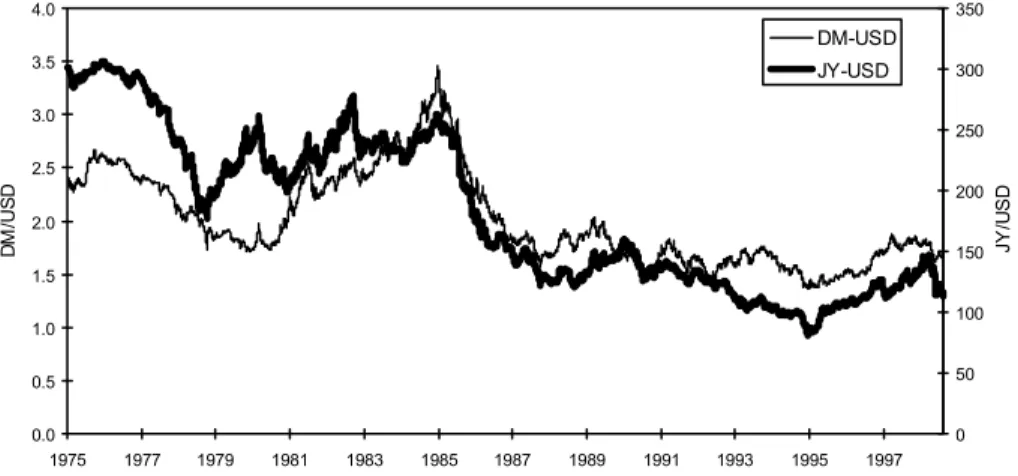
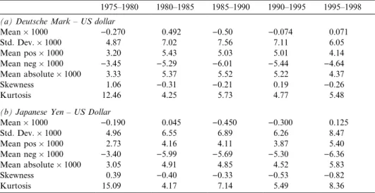
Technical analysis generates profits by accurately predicting trends in exchange rates and in Fig. 1 we see periods of long upward and downward movements in both currency pairs. The dollar appreciated against the Mark from 1980 to 1985, depre- ciated from 1985 to 1987, and was relatively stable from 1987 to 1998. Relative to the yen, the dollar was stable from 1980 to 1985, depreciated rapidly from 1985 to 1987 and was stable again from 1987 to 1998. Table 1 presents some descriptive sta- tistics for the log first differences (continuously compounded returns) of the bid for these two currency pairs. The returns display the well-known characteristics of ex- change rates – low skewness, large kurtosis, very little autocorrelation, and the pres- ence of conditional heteroskedasticity. Except for the mean, these characteristics were stable over time: the mean is positive or negative reflecting the appreciation or depreciation of the currencies in the different periods. Interestingly the average absolute value of returns was stable over time.

0.0 0.5 1.0 1.5 2.0 2.5 3.0 3.5 4.0

1975 1977 1979 1981 1983 1985 1987 1989 1991 1993 1995 1997

DM/USD

0 50 100 150 200 250 300 350

JY/USD

DM-USD JY-USD

Fig. 1. Exchange Rates from 1975 to 1998. Graph of the daily bid exchange rate for the DM-$, and Yen-$

over the period from January 1, 1975 to December 31, 1998. The data was obtained from DRI and is the New York opening from Bank America (San Francisco) until 1986 and the London close from NatWest (London) afterward.

Fig. 2 illustrates the changing nature of intervention activity over the period from 1980 to 1998. In Fig. 2(a) and (b) we see that the Fed was fairly active in both the DM-$ and Yen-$ markets from 1980 to mid-1981, inactive from mid-1981 to 1987 (except for some selling of dollars in late-1985), it returned between 1987 and 1995 and was absent from mid-1995 until the end of our sample. On the other hand Fig. 2(c) and (d) show the Bundesbank was very active in both the DM-$ and the DM-European currency markets from 1980 until it ceased intervention activities in mid-1995. These interventions were clustered with the Bundesbank intervening in the DM-$ market almost twice as often as the Fed: the Fed or the Bundesbank intervened on 8% and 17% of trading days respectively, yet if there was an interven- tion on the previous day these percentages increased to 57% and 60% (the average duration of intervention episodes was 2.6 and 2.8 days respectively).

The average size of interventions increased over the sample and both Central BanksÕ interventions remained similar in size in each sub-period. As a result of the Bundesbank being more active early in the sample, the overall average size of Bun- desbank interventions was smaller than Fed interventions ($77M versus $124M).

Comparing types of interventions, announced interventions were, on average, almost twice as large as the unannounced ⁷(in the DM-$ market $197M for the Fed and

Table 1

Summary statistics for exchange rate returns

1975–1980 1980–1985 1985–1990 1990–1995 1995–1998 (a) Deutsche Mark – US dollar

Mean1000 )0.270 0.492 )0.50 )0.074 0.071

Std:Dev:1000 4.87 7.02 7.56 7.11 6.05

Mean pos1000 3.20 5.43 5.03 5.01 4.14

Mean neg1000 )3.45 )5.29 )6.01 )5.44 )4.64

Mean absolute1000 3.33 5.37 5.52 5.22 4.37

Skewness 1.06 )0.31 )0.21 0.19 )0.26

Kurtosis 12.46 4.25 5.73 4.77 5.48

(b) Japanese Yen – US Dollar

Mean1000 )0.190 0.045 )0.450 )0.300 0.125

Std:Dev:1000 4.96 6.55 6.89 6.26 8.47

Mean pos1000 2.73 4.16 4.11 3.87 5.40

Mean neg1000 )3.40 )5.99 )5.69 )5.30 )6.36

Mean absolute1000 3.05 4.91 4.85 4.52 5.83

Skewness 0.39 )0.40 )0.33 )0.53 )0.82

Kurtosis 15.09 4.17 7.14 5.49 8.36

Summary statistics for the continuously compounded (or log returns) of the daily bid DM-$, and Yen-$

spot exchange rates from January 1, 1975 to December 31, 1998. The data was obtained from DRI and is the New York opening from Bank America (San Francisco) until October 8, 1986 and the London close from NatWest (London) afterward.

7This is consistent with the results of Klein (1993) who found Fed interventions announced in newspapers were larger than the unannounced. Further we find the interventions announced in both the newspaper and the newswire were slightly larger than those that were only announced on the newswire.

(a)

(b)

-1.000 -500 0 500 1.000 1.500

1980 1980 1981 1982 1983 1984 1985 1986 1987 1988 1989 1990 1991 1992 1993 1994 19 95 1996 1997 1998

-1.000 -500 0 500 1.000 1.500

1980 1980 1981 1982 1983 1984 1985 1986 1987 1988 1989 1990 1991 1992 1993 1994 1995 1996 1997 1998

(c)

(d)

-2.500 -2.000 -1.500 -1.000 -500 0 500 1.000 1.500

1980 1980 1981 1982 1983 1984 1985 1986 1987 1988 1989 1990 1991 1992 1993 1994 1995 1996 1997 1998

-10.000 -8.000 -6.000 -4.000 -2.000 0 2.000 4.000 6.000 8.000 10.000

1980 1980 1981 1982 1983 1984 1985 1986 1987 1988 1989 1990 1991 1992 1993 1994 1995 1996 1997 1998

Fig. 2. Timing and Quantity of Federal Reserve and Deutsche Bundesbank Interventions 1980–1998.

Graph of the daily quantity of official Central Bank intervention by the Federal Reserve and the Deutsche Bundesbank over the period from January 1, 1980 to December 31, 1998. The quantities are in millions of US dollars and millions of Deutsche Marks respectively. (a) Interventions by the Federal Reserve in the DM-$ market: (b) Interventions by the Federal Reserve in the Yen-$ market: (c) Interventions by the Deutsche Bundesbank in the DM-$ market: (d) Interventions by the Deutsche Bundesbank in the DM- ERM market (interventions in the European currencies):

$105M for the Bundesbank versus $98M and $55M respectively) but coordinated were only slightly larger than unilateral interventions. The frequency also varied:

about 65% of interventions were unannounced, less than 25% of all interventions were coordinated, but coordinated interventions were over twice as likely to be an- nounced than unilateral. As a result it does not appear that all interventions are cre- ated equal, but it is not clear what impact this has on technical trading returns.

3. Technical trading rules

This section discusses the technical trading strategies we consider. Because imple- menting technical trading strategies generally requires skill, judgment and other characteristics that are difficult to mimic, we consider one of the simplest and most objective trading strategies: moving average trading rules.⁸This rule generates a buy or sell signal by comparing the current exchange rate to a moving average of past exchange rates: buy when the current spot price is above the moving average and sell when it is below. For example, at time t theT-day moving average of the spot ex- change rate (st) is defined to be:

MAðTÞ_t¼1 T

X^T1

i¼0

s_ti: ð1Þ

With the current spot price defined in DM/US$, for example, this means the trader wants to be long dollars whens_tPMAðTÞ_t.

Although many studies ignore transaction costs, we use continuously com- pounded returns that account for the costs associated with the implementation of these trading strategies. These include buying at the quoted ask and selling at the bid. This provides a conservative estimate of the actual costs (Goodhart et al.

(1996) found that quoted prices are 2–3 ticks wider than actual transaction prices).

Because we assume investors borrow the currency they sold and invest the currency they are holding at the corresponding overnight interest rates, ⁹the strategies are self-financing and the returns are excess returns. Formally the returns are calculated as follows:

when the investor maintains the same position from time tto timetþ1:

long dollarsr_t¼ flnðs^A_tþ1=s^A_tÞ þln½ð1þi^A_t Þ=ð1þi^B_tÞg; ð2aÞ short dollars rt¼ ð1Þflnðs^B_tþ1=s^B_tÞ þln½ð1þi^B_t Þ=ð1þi^A_tÞg; ð2bÞ when the investor changes position:

8Neely et al. (1997) consider more complex trading strategies and find that the optimal technical trading strategies over a similar time period were slight modifications of this trading rule.

9The overnight interest rates and the exchange rates are not quoted at exactly the same time, so it may not be possible to obtain the exact returns calculated here. However the interest rates play such a minor role in the trading rule returns that this should not significantly influence our results.

long to short rt¼ flnðs^B_tþ1=s^A_tÞ þln½ð1þi^A_t Þ=ð1þi^B_tÞg; ð2cÞ

short to long r_t¼ ð1Þflnðs^A_tþ1=s^B_tÞ þln½ð1þi^B_t Þ=ð1þi^A_tÞg; ð2dÞ where fs^A_t;s^B_tg are the quoted ask and bid for the spot DM-$ rate at time t, and fi^A_t;i^B_tg andfi^A_t ;i^B_t g are the quoted ask and bid for the overnight US and German interest rates respectively.¹⁰

3.1. Profitability of technical analysis

Table 2 presents the returns from different moving average trading strategies.

Over the entire period, the returns for the DM-$ are generally statistically different from zero – t-statistics of between 1.3 and 2.5. The returns in the Yen-$ market are all statistically significant witht-statistics ranging from 2.7 to 3.7. As a conse- quence of the moving average trading rules generating statistically significant returns over the out-of-sample 1975–1980 period as well, the concern of ex-post bias in our choice of trading strategies is minimal. In fact it is only in the final sub-period that the statistical significance of the returns in the DM-$ and Yen-$ market vanishes.

The concentration of profitability in the 1975–1995 period suggests a possible role for Central Bank intervention in the apparent inefficiency of the foreign exchange market.

Many researchers ignore transaction costs because ‘‘buying or selling $1 will cost the trader about $0.00025’’ (Neely, 1998), so we investigate the sensitivity of our trading rule returns to transaction costs. In Table 3 we start with no transaction costs – the returns are the log first difference of the midpoint of the spot exchange rate. Next we replace the midpoints with the corresponding bid and ask values. Fi- nally we add the cost or benefit from the overnight investment in each currency. The impact of these transaction costs on our returns can be most clearly seen for the MA(10) trading rule which changes position often thus incurring these costs the most frequently. In the simplest case, without any transaction costs, the MA(10) trading rule generates returns with t-statistics of 3.32 in the DM-$ market for 1980–1998.

This falls to 1.77 when the bid–ask spread is accounted for and to 1.74 with the in- clusion of overnight investing. Other than for the MA(10) trading rule, this table demonstrates that transaction costs do not play a major role in the statistical signif- icance of our technical trading returns. As a consequence it is unlikely that the prof- itability of our technical trading strategies is the result of market frictions such as transaction costs.

10For example, if we assume the trading rule directs the trader to buy DM the trader starts by borrowing dollars at the overnight US interest rate ask. The dollars are converted to DM at the spot bid and invested at the overnight German interest rate bid. The next day the trader either continues to hold DM and rolls over the overnight positions, or reverses them to hold dollars. Consequently the trader earns a dollar return defined as the product of the overnight German interest rate and the appreciation of the DM, less the interest to borrow dollars.

3.2. Significance of the trading rule returns

The previous discussion relied upont-statistics to assess the statistical significance of our trading returns. This requires assuming the mean of the trading returns is as- ymptotically normally distributed. The results in Table 1 suggest this may be a prob- lem. To estimate the impact of this assumption on our results, we use a bootstrap to non-parametrically estimate the statistical significance of our trading rule returns.

Our bootstrap methodology is similar to that outlined in Brock et al. (1992). We start by generating bootstrapped exchange rate series under the null hypothesis that the foreign exchange market is efficient and characterized by different random walk processes (for details please see Appendix A). A sample of the bootstrappedp-values is presented in Table 4. These values suggest that thet-statistics provide reasonable estimates for the statistical significance of our technical trading returns. For exam- ple, the t-statistic for the returns from the MA(150) trading rule implied a p-value of 0.007. This compares very well to the bootstrapped p-values of 0.007 and 0.012 obtained under each of the random walk models. Since thet-statistics are easily com- puted and provide a reliable measure of statistical significance, we rely on them in the subsequent analyses.

Table 2

Statistical significance of technical trading rule returns

Lags 1980–1998 1975–1980 1980–1985 1985–1990 1990–1995 1995–1998 (a) For the DM-$

10 1.74 2.13 1.65 2.37 1.10 0.55

25 1.33 3.07 2.70 2.20 2.13 0.26

50 2.18 3.64 2.94 2.55 1.68 1.34

75 1.41 2.47 2.15 2.10 2.02 0.67

100 1.85 2.67 2.23 2.21 2.04 0.54

125 2.23 2.86 2.30 1.60 2.20 0.64

150 1.72 2.36 2.10 1.23 1.85 0.43

200 1.90 2.41 2.11 0.70 1.83 0.42

250 2.52 2.61 1.89 0.65 1.56 )0.05

(b) For the Yen-$

10 2.73 1.96 1.09 1.44 2.59 )1.00

25 3.12 2.68 1.66 1.22 2.29 )0.56

50 3.06 3.67 2.73 1.62 2.44 0.50

75 3.49 4.33 3.22 0.71 3.09 0.77

100 3.70 4.49 3.27 1.39 2.34 1.00

125 3.47 4.26 3.19 1.54 2.25 1.14

150 3.18 4.00 3.00 1.41 2.05 0.86

200 2.95 3.24 2.34 1.14 1.88 )0.05

250 2.90 2.90 1.91 0.23 1.18 0.01

Thet-statistics from the DM-$ and Yen-$ returns generated by different moving average trading rules. The returns are calculated using formulas (2a)–(2d). The exchange rates were obtained from DRI and are the New York opening from Bank America (San Francisco) until October 8, 1986 and the London close from NatWest (London) afterward. The German and Japanese overnight interest rates were obtained from DRI and the US interest rates from the Federal Reserve.

The statistical significance of technical trading returns does not tell us whether the returns adequately compensate investors for the risk of investing in the foreign ex- change market. Ideally we would answer this question by comparing the trading rulesÕ returns to the required return for investing in this market. Because standard asset pricing models perform poorly in the foreign exchange market (see Lewis, 1995 for a discussion), we compare the returns from technical analysis to those from investing in a risk-free asset (one-month US Treasury bills) and in a risky asset (the S&P500). Investing in US T-Bills over this period would have generated an average annualized return of 7.0% and investing in the S&P500 an average annualized return of 18.6%, or an average annualized excess return of 11.6%. To compare the risk-re- ward trade-off across these investment strategies we use one-year Sharpe Ratios – a higher Sharpe Ratio indicates an investment with a better risk-reward trade-off.¹¹ Over our sample period, the one-year Sharpe Ratios for investing in the S&P500 and the MA(150) trading rule were 0.49 and 0.65 respectively (from 1980 to mid- 1995 they were: 0.34 and 0.76 respectively). This suggests technical trading strategies provide an attractive return for their risk.

In summary, technical trading strategies generate both statistically and economi- cally significant profits. The decrease in their significance after 1995 is consistent with

Table 3

Impact of transaction costs on technical trading rule returns

Lag 1980–1998 1975–1980

No trxn costs

Trxn costs no int rates

Trxn costs int rates

No trxn costs

Trxn costs no int rates

Trxn costs int rates

10 3.32 1.77 1.74 3.45 2.11 2.13

25 2.80 1.37 1.33 3.32 2.88 3.07

50 2.29 2.20 2.18 3.75 3.61 3.64

75 1.59 1.43 1.41 2.61 2.38 2.47

100 2.25 1.89 1.85 2.78 2.65 2.67

125 2.27 2.25 2.23 2.95 2.91 2.86

150 1.87 1.74 1.72 2.37 2.32 2.36

200 2.06 1.94 1.89 2.46 2.37 2.41

250 2.51 2.54 2.51 2.56 2.58 2.61

The values in this table for the DM-$ returns using different moving average trading rules from 1975 to 1998. The returns are calculated using formulas (2a)–(2d). The DM-$ exchange rates were obtained from DRI and are the New York opening from Bank America (San Francisco) until October 8, 1986 and the London close from NatWest (London) afterward. The German overnight interest rates were obtained from DRI and the US interest rates from the Federal Reserve. The first column contains thet-statistics for returns using only the midpoint of the exchange rate and no overnight investing (e.g. without any transaction costs), next the returns including the transaction costs based on the quoted bid and ask but no overnight investing and the third column for the returns incorporating both the bid–ask transaction costs and investing overnight.

11The one-year Sharpe ratios are estimated using: ffiffiffiffi pN

ðl_return=r_returnÞwhere l_return is the average continuously compounded daily excess return from each investment;rreturn, the standard deviation;andN, the number of trading periods in one year.

the hypothesis that this apparent inefficiency could be related to Central Bank inter- vention activities – a decrease in intervention activity is one of the main differences between these periods.

4. Vector autoregression analysis

To estimate the relationships between exchange rate movements and different eco- nomic factors, especially interventions, we use a VAR model to determine whether past values of one variable, v, are linearly informative about the current value of another variable,x:

x_t¼b₀þX^p

i¼1

b_1ix_tiþX^p

i¼1

b_2iv_tiþet ð3Þ

This is a form of Granger causality test (see Hamilton, 1994 for a discussion) where the null hypothesis is that the past values ofvdo not help explain the present value of

Table 4

Non-parametric estimations of the significance of technical trading rule returns Parametric esti-

mate of the p-values from

Non-parametric estimates of the p-values from

t-Statistic H0: random walk process 1

H0: random walk process 2

Trading rule MA(10) 0.001 0.000 0.000

MA(50) 0.002 0.004 0.007

MA(150) 0.007 0.007 0.012

MA(250) 0.088 0.088 0.093

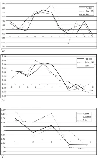
Removing these interven- tions from MA(150)

Fed DM 0.169 0.247 0.253

Fed JY 0.053 0.063 0.088

all Fed (DM/JY) 0.206 0.216 0.242

Buba in USD 0.363 0.421 0.413

Buba in ERM 0.052 0.052 0.069

all Buba (US/

ERM)

0.500 0.516 0.524

Both US-DM 0.106 0.122 0.141

The values in this table are for thep-values of the different trading rule returns over the period from 1980 to 1998. These are implied from the parametrically determinedt-statistics in the first column of values and from a non-parametric bootstrap in the second and third columns (see Appendix A for a discussion and the definitions of the two random walk processes). They were calculated using formulas (2a)–(2d). The exchange rates were obtained from DRI and are the New York opening from Bank America (San Francisco) until October 8, 1986 and the London close from NatWest (London) afterward. The German overnight interest rates were obtained from DRI and the US interest rates from the Federal Reserve. The bottom portion of the table verifies the measures of statistical significance of trading rule returns used in the replication of LeBaronÕs (1999) analysis performed in Section 5. The replication of LeBaron (1999) involves the calculation of returns for the trading rules after removing days on which the specified central bank intervention activities occurred.

xor formallyH₀:b₂₁¼b₂₂¼b₂₃¼b₂₄¼b₂₅¼0. The number of lags,p, was chosen using the Akaike information criteria (AIC). The test statistic for our null hypothesis is obtained by comparing the sum of squared errors from the unconstrained re- gression in Eq. (3) (called SSEu) to the sum of squared errors from a regression using only the lagged values ofx(called SSEc). Both of these models can be estimated by ordinary least squares. The test statistic is defined as:

G_t¼ ðSSEcSSEuÞ

SSEu=ðT ð2pÞ 1Þ ð4Þ

This follows an F-distribution under the assumption that SSEc and SSEu are as- ymptotically normally distributed.¹²IfG_tis greater than the critical value we reject the null hypothesis that past values ofvdo not provide information relevant to the current value ofx. Cooley and LeRoy (1985) suggest this technique for determining whether changes in one variable systematically precede changes in another.

We use this technique to investigate the possible correlations between technical trading profits, Central Bank interventions, market uncertainty and monetary pol- icy. We consider measures of market uncertainty because increased market uncer- tainty could lead to central bank intervention (Cross, 1998) or possibly indicate the presence of a risk premium. We consider monetary policy because many models suggest that it may influence exchange rates (see Frankel and Rose, 1995) or be in- fluenced by exchange rate movements (e.g. Kaminsky and Lewis, 1996). As a result the main hypotheses we investigate are: How is uncertainty related to trading rule profitability? Interventions? Do changes in monetary policy precede trading rule profitability? Do changes in monetary policy precede or follow interventions?

4.1. Interventions, exchange rates and trading rule returns

In the first and fourth columns of Table 5a we see the relationships between the continuously compounded returns for the DM-$ and Yen-$ exchange rates and dif- ferent economic factors.¹³ We start with the G_t-statistics for the DM-$ exchange rate. The only measures of market uncertainty that appear to have predictive power for changes in the exchange rate are the average volume and the differences in the volume and open interest between the at-the-money put and call options. Moving to our intervention variables, we find interventions by the Federal Reserve in the DM and Yen had predictive ability for movements in the daily DM-$ exchange rate G_t-statistic values of 3.04 and 2.33 respectively). Because interventions are clustered

12Because this is an asymptoticF-test, Geweke et al. (1983) and Guilkey and Salemi (1982) investigate the finite sample properties of this statistic. They find that it is robust to changes in the number of lagged values, the presence of serial correlation in the variables and other deviations from normality (even if the chosen parameterization was not correct).

13The results in Table 5 use a lag length of five days. Although the optimal lag lengths obtained using the AIC varied from 2 to 20, the most common value was 5 and the significance of the results was consistent using the optimal lag length or 5. Consequently, to aid in interpretation of the results we use five lags throughout.

Table 5

Results from the VAR analysis

Variable DM-$ JY-$

FX return

Abs(FX returns)

Trading rule

FX return

Abs(FX returns)

Trading rule Panel (a)

Spread in DM-$ 1.16 0.96 1.01 1.94 1.55 2.29

Spread in JY-$ 0.81 2.04 1.42 0.58 1.29 0.86

Forward premium DM-$ 1.63 1.00 0.81 0.38 0.78 0.62

Forward premium JY-$ 1.25 0.11 1.19 2.38 1.90 2.52

Volatility (previous week) 1.23 10.65 1.11 1.92 4.55 1.71

Implied volatility 1.55 3.77 1.56 0.96 1.75 0.96

Open interest 1.34 0.98 1.29 0.32 1.61 0.29

Volume 2.34 1.79 2.36 1.05 1.58 1.08

Put–call volume 4.60 2.44 1.39 2.62 1.80 0.46

P–C open int 2.26 0.52 0.68 0.97 2.10 0.40

P–C implied volatility 1.34 1.76 1.44 0.68 1.07 0.58

Fed interventions in DM 3.04 3.99 0.84 0.82 1.93 1.08

Announced Fed in DM 2.18 1.65 0.81 0.77 0.72 1.34

Fed interventions in Yen 2.33 0.76 0.76 0.75 1.18 2.52

Announced Fed in Yen 1.69 0.47 1.15 0.77 1.22 2.31

Bundesbank interventions in $ 1.06 2.16 2.28 0.22 1.23 0.84

Announced Bundesbank in $ 1.11 1.32 1.16 0.59 0.77 0.42

Fed–Bundesbank in DM-$ 1.31 2.11 2.35 0.94 2.65 0.96

Announced Fed–Buba in DM-$

0.90 0.81 0.46 0.87 0.31 0.92

Announced Bank of Japan 0.79 1.41 0.79 1.09 0.51 0.87

US short-term rates 0.55 1.04 0.51 0.04 0.79 0.05

German short-term rates 0.71 1.31 0.71 0.68 0.97 0.69

S.Sapp/JournalofBanking&Finance28(2004)443–474

Japanese short-term rates 0.83 1.13 0.77 2.85 3.65 2.84

Beginning Fed in DM 2.66 1.27 0.98 2.04 0.45 1.34

Beginning Fed in JY 1.32 0.91 1.42 1.30 0.84 2.18

Beginning Buba in USD 1.13 0.50 0.69 1.37 0.69 0.46

Beginning Fed–Buba 2.60 2.53 1.37 2.28 2.23 1.05

End Fed in DM 0.94 2.03 1.60 0.92 2.36 0.71

End Fed in JY 1.15 0.63 1.37 1.55 0.76 0.99

End Buba in USD 0.45 0.57 0.28 0.85 0.66 0.32

End Fed–Buba in USD 0.73 0.47 2.71 1.32 0.86 0.52

Panel (b)

Fed DM

Fed JY Bundes- bank USD

Both USD

Announced Fed DM

Announced Fed JY

Announced Bundes- bank USD

Announced both USD

Announced Bk of Japan USD

FX Return 4.36 6.06 9.23 5.00 5.03 5.70 6.59 1.72 1.70

Abs(Return) 1.24 1.05 1.30 1.86 2.51 2.64 2.72 1.51 2.25

Trading rule 2.48 2.08 5.93 2.34 2.00 2.89 3.52 1.81 1.15

Spread in DM-$ 2.93 1.38 8.79 4.33 1.32 0.87 3.32 1.37 2.12

Spread in JY-$ 3.34 1.61 6.26 3.79 1.95 0.83 3.39 1.45 3.04

Forward premium DM-$ 2.75 0.63 9.37 4.21 0.32 0.16 1.86 0.11 0.14

Forward premium JY-$ 0.43 0.13 2.97 1.49 0.21 0.46 0.62 0.34 0.47

Volatility (previous week) 0.49 0.68 0.37 0.53 0.85 1.79 2.84 1.04 0.68

Open interest 7.40 8.03 2.09 7.47 9.11 7.47 3.83 3.84 4.40

Volume 2.89 2.27 2.27 2.31 4.69 2.38 1.14 1.62 1.26

Implied volatility 1.56 1.32 3.48 2.34 1.14 0.57 1.58 1.69 1.67

P–C open interest 10.01 2.81 2.11 6.35 8.74 2.70 1.86 2.10 0.30

P–C volume 2.36 0.61 0.98 1.53 2.24 0.51 1.05 0.95 1.11

P–C implied volatility 1.51 1.34 3.70 2.96 1.08 0.84 1.83 1.77 2.32

US short-term rates 0.47 0.09 0.87 0.55 0.14 0.23 0.53 1.07 1.20

German short-term rates 1.24 1.17 0.77 0.26 1.26 0.94 1.40 0.99 0.55

Japanese short-term rates 0.55 0.75 1.41 0.81 1.00 1.28 0.09 0.43 0.61

S.Sapp/JournalofBanking&Finance28(2004)443–474457

Panel (c)

Ger- man S- T Rate

German Def Prem

DM- USD spread

DM- USD historic volatility

DM-USD implied vol- atility

Japanese S-T rate

Japanese Def Prem

JY-USD spread

JY-USD historic vol- atility

JY- USD implied volatil- ity

Spot rate 1.21 0.43 3.85 1.46 4.02 1.23 0.12 0.34 8.20 0.62

Abs(spot) 1.04 0.72 1.24 350.52 2.52 2.92 0.23 0.65 342.80 0.43

Trading rule 0.56 0.44 4.05 1.17 4.09 1.16 0.88 0.44 10.90 0.82

Fed DM 0.85 0.15 0.68 3.24 0.93 0.69 0.08 1.75 2.35 3.04

Fed JY 0.85 0.00 0.52 1.69 1.65 1.05 0.00 1.58 2.39 0.02

Buba USD 2.53 3.87 5.78 4.62 0.30 0.40 2.04 3.98 1.43 0.14

Both DM-USD 2.98 6.20 0.83 8.48 0.53 0.37 3.15 0.89 2.55 1.19

Ann Fed DM 0.62 0.00 1.53 2.62 1.15 0.49 0.00 0.53 1.00 5.03

Ann Fed JY 0.61 0.00 1.66 2.04 1.73 0.69 0.00 1.18 2.56 0.02

Ann Buba USD 2.11 0.01 1.49 2.86 0.25 0.35 0.00 0.59 1.16 0.14

Ann both USD 0.98 0.00 1.74 1.87 0.38 0.29 0.00 0.81 0.37 4.11

Ann B of J 0.65 0.04 1.10 1.05 0.97 0.28 0.00 0.63 1.57 2.57

Start Fed DM 0.84 0.23 2.21 1.22 0.94 1.04 0.11 1.65 0.49 0.53

Start Fed JY 0.91 0.00 0.53 1.64 2.01 1.23 0.00 1.27 0.70 0.01

Start Buba USD 1.52 0.02 3.43 6.06 0.19 0.61 0.00 3.78 1.00 0.27

Start both 2.63 8.70 0.84 8.58 0.78 0.45 4.42 0.67 1.63 1.68

End Fed DM 0.50 0.24 1.30 0.69 1.04 1.07 0.13 1.81 0.61 0.13

End Fed JY 0.44 0.00 0.83 1.30 2.41 1.11 0.00 2.00 0.99 0.01

End Buba USD 2.37 0.06 3.21 2.10* 0.23 0.35 0.00 3.25 2.17 0.48

End both USD 1.91 9.43 0.73 1.59 0.60 0.50 4.78 0.83 1.60 1.75

Panel (a): The values in this table are for theG_t-statistics (Eq. (4)) from the tests of Eq. (3) over the period from 1980 to 1998. The values are for the log first differences (continuously compounded returns), the absolute value of these returns and the returns from the 50 day moving average trading rules. The data sources are discussed in Section 2. (Note: indicates statistical significance at the 10% level or better and indicates statistical significance at the 5% level or better.)

Panel (b): The values in this table are for theGt-statistics (Eq. (4)) from the tests of Eq. (3) over the period from 1980 to 1998. The values are for the absolute value of the official interventions by the Federal Reserve and Deutsche Bundesbank. The exchange rates are from DRI (the New York opening from Bank America (San Francisco) until October 8, 1986 and the London close from NatWest (London) afterward. (Note: indicates statistical significance at the 10% level or better and indicates statistical significance at the 5% level or better.)

Panel (c): The values in this table are for theGt-statistics (Eq. (4)) from the tests of Eq. (3) over the period from 1980 to 1998. The values are for our measures of market uncertainty: the bid–ask spread and the standard deviation of the exchange rates over the past week and past month with exchange rates from DRI (the New York opening from Bank America (San Francisco) until October 8, 1986 and the London close from NatWest (London) afterward). (Note: indicates statistical significance at the 10% level or better and indicates statistical significance at the 5% level or better.)

S.Sapp/JournalofBanking&Finance28(2004)443–474

and it is possible that the market reaction to the beginning of intervention activity is different from other days, especially the end, we consider the first and last days of intervention activity separately. In the bottom part of the table, we present the re- sults for only the first and last days of interventions. We find that the significance of Fed interventions in DM are concentrated on the first day of intervention activity in the DM and the first day of coordinated Fed–Bundesbank intervention activity (values of 2.66 and 2.60 respectively). This suggests that it is the beginning of the in- tervention episode that provides the most statistically significant information to pre- dict future exchange rate movements. Analyzing the announced interventions, we find the announced Fed interventions in DM were correlated with DM-$ returns (value of 2.18). This suggests the market reacts to the signal contained in the announcement.¹⁴For the Yen, the statistically significant relationships with changes in monetary policy (changes in the forward premium and short-term interest rates) differences in the trading volume of put and call options and the first days of Federal Reserve intervention in the DM-$ market.

The second and fifth columns consider how the absolute value of the foreign ex- change returns are related to our set of economic factors including the absolute value of interventions. We use the absolute value of interventions because this allows us to analyze the relationship between changes in returns and interventions without having to consider the direction (e.g. returns are larger around interventions, whether or not it is an upward or downward movement or an intervention to support or weaken the dollar). For the DM-$, we see that changes in market uncertainty con- sistently precede movements in the exchange rates (value of over 10 on our historical measure of exchange rate volatility and 3.77 on the average implied volatility). The relationships are also significant for the Fed and Bundesbank interventions in the DM-$ market. For the Yen we find similar relationships except that for the Yen the value of the Japanese Short-term interest rates also plays a significant role.

The final part of Table 5a investigates the technical trading returns in both cur- rencies (columns three and six). The returns are for the MA(50) trading rules against our set of economic factors and the absolute value of interventions.¹⁵Overall these results indicate that interventions have the most significant predictive power for tech- nical trading returns. For the DM-$ trading rules, it was unilateral interventions by the Bundesbank and coordinated Fed–Bundesbank interventions that were the most significant but for the Yen it was Fed interventions in Yen. Although the last day of an episode of intervention activity had the most predictive power for technical trad- ing returns in the DM-$ it was the first day for Yen. Across trading rules (results not presented) changes in market uncertainty had more significant predictive ability for the returns of the shorter trading rules, but for the longer moving average trading rules it was the Central Bank intervention activities. For the Yen-$ trading rules,

14Another argument is that the announcement was based on rumors related to other factors that generated the movements in exchange rates. This is highlighted in results not presented that demonstrate the effect of announced Fed interventions in DM was largest on days of incorrectly announced interventions.

15The results for the other trading rules are very similar so they are not presented.