central Mexico, southern Peru, and southwest Japan

The lateral extent of the USL is used as a constraint on the nature of the flat-to-normal transition in central Mexico (Chapters 2 and 3) and southern Peru (Chapter 4). In Chapter 2, I study the fine-scale seismic structure of the central Mexico subduction zone along the western transition from flat to normal subduction.

Figure 1.1: Map showing study locations in central Mexico (blue box), southern Peru (red box), and southwest Japan (green box)

Abstract

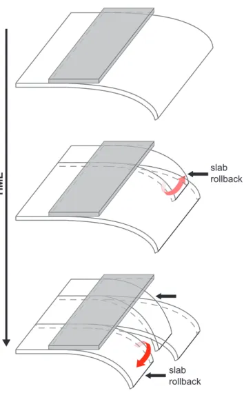
We suggest that the Cocos plate is currently fragmenting into a North Cocos plate and a South Cocos plate along the projection of the OFZ, consistent with observations of variable Cocos plate motion on either side of the OFZ. This rifting event may be a young analogy to the 10 Ma Rivera-Cocos plate boundary, and may be related to the rollback of the plate in central Mexico.

Introduction

The rifting of the slab may provide a shortcut mechanism related to the trench-parallel flow associated with the rollback of the slab in central Mexico (Russo and Silver, 1994; Ferrari, 2004). We perform 1D and 2D waveform modeling to image the structure of the slab and overriding plate.

Data Analysis

Data

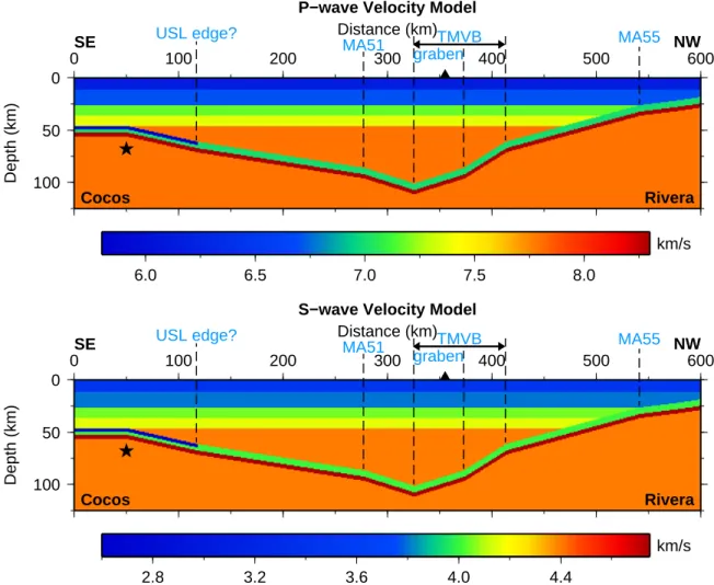
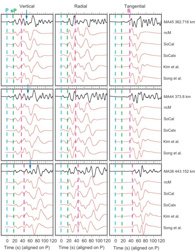
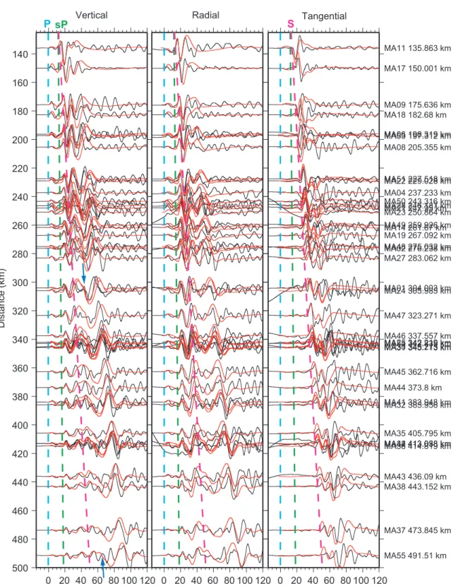
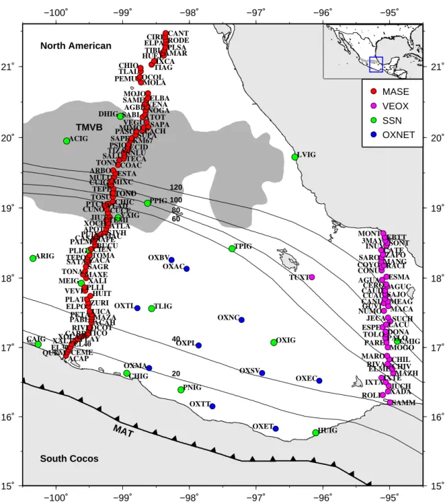
The receiver function results from Kim et al. (2010) are used to constrain the depth of the Moho to 45 km in the SoCalx and ncM models. A NW-SE trend profile across the MARS array (see Figure 2.1 for location) of the ncM.

Figure 2.1: Map showing the MARS stations (blue dots) and events (stars, focal mechanisms) used in this study

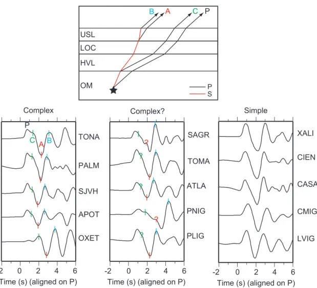
Ultra-slow Velocity Layer

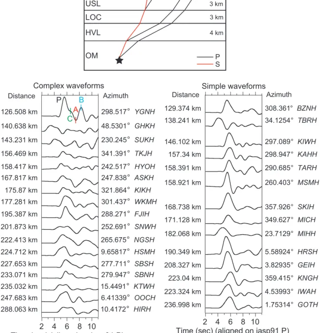
For stations located within the TMVB, complexities in the waveforms are observed after the S-wave arrival in the data (indicated by the orange box) and are not predicted by the model. All three of these phases are visible in the complex waveforms within 4 seconds of the P wave.

Figure 2.3: Comparison of 1D modeling results of event 3 for the five models tested at three stations.

Seismicity and Slab Dip Across USL Edge

Discussion

The proposed fragmentation of the Cocos Plate along the OFZ is an example of this process. This test passed at a risk level of 5%, indicating that the movement of the Cocos Plate north of the OFZ is different from that to the south (Bandy et al., 2000).

Figure 2.12: 3D schematic of the two-tear model illustrating the geometry of the S Cocos, N Cocos, and Rivera plates, along with the Orozco (OFZ; young tear) and Rivera (RFZ; old tear) fracture zones

Conclusions

Supplemental Figures

McNally (1984), Seismicity and tectonics of the Rivera plate and implications for the 1932 Jalisco, Mexico, earthquake, J. Pardo (1993), Geometry of the Benioff zone and stress state in the overriding plate in central Mexico, Geophys.

Figure 2.13: 1D modeling results of event 3 for the SoCal velocity model filtered to 0.01–0.1 Hz.

Abstract

This potential rift, along with rifting along the Orozco Fault Zone to the northwest, suggests a slab rollback mechanism in which separate slab segments move independently, allowing mantle flow between segments.

Introduction

The abrupt rotation of trench-parallel SKS fast directions to trench-perpendicular near a plate tear (or a circular pattern of anisotropy around a plate edge) indicates 3D toroidal flow of mantle material through the gap (Peyton et al., 2001; Kneller and van Keken, 2008 ; Zandt and Humphreys, 2008 ), which has important implications for rollback of the subducted slab. The addition of this less dense asthenosphere to the wedge would also increase the rollback of the plate segment (Schellart et al., 2007; Soto et al., 2009). Based on structural modeling results and seismic and tectonic observations in the west, Dougherty et al.(2012) suggested that the Cocos plate is currently fragmenting into a North Cocos plate and a South Cocos plate.

Tectonic Setting

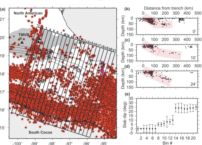
The direction of convergence of the South Cocos plate near the Middle America Trench (MAT) is indicated by the black arrow (DeMets et al., 2010). This tearing is suggested to indicate an ongoing fragmentation of the Cocos plate into the N Cocos and S Cocos plates, respectively (Dougherty et al., 2012). The previously identified location of the O'Gorman Fracture Zone is also shown (red dashed line).

Figure 3.1: Map showing the locations of MASE, VEOX, SSN, and OXNET stations along with events (stars, focal mechanisms) used in this study

Data Analysis

Data

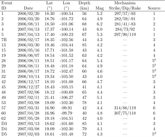
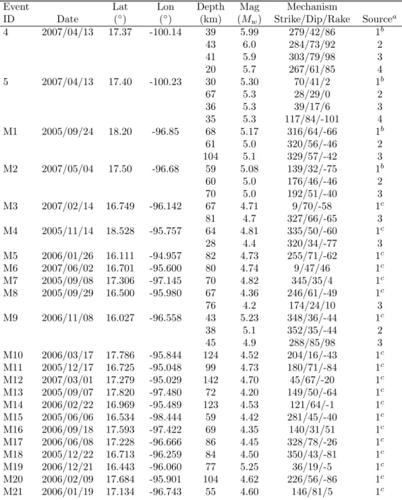
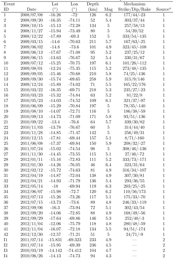
Instead, Kanjorski (2003) identified several parallel ridges consisting of small to medium-sized (up to ~20 km diameter and 1700 m high) seamounts generated as off-axis volcanism entering the MAT in this region, with the larger seamounts the mountains remained physically intact throughout the subduction process (Figure 3.2b). Included in this zone is the Puerto Escondido submarine cluster, a broad volcanic feature dotted with > 100 volcanic cones and accompanying lava flows (Figure 3.2) (Kanjorski, 2003). Lat Lon Depth Mag Mechanism Event. aSources are 1) focal mechanism, Mw and depth from this study;.

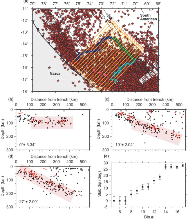
Table 3.1. Events used in eastern central Mexico and their source parameters.

Slab Dip

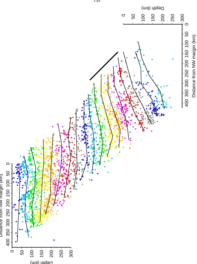
Data in twenty-one 25 km wide bins, roughly perpendicular to the MAT, are analyzed for plate depth changes in this region. Note the significant change in the plate dip between bins 13 and 14. e) Draw the plate dip over the data bins. The estimated mat depth in each of the twenty-one bins is shown in Figure 3.3e.

Ultra-slow Velocity Layer

Simple waveforms lack the shoulder in the direct P pulse representative of the C phase and also have uncharacteristically shaped and/or low amplitude A and B phases, indicating that no USL is present. Note that the boundary between the USL and no USL zones roughly coincides with the eastern end of the TMVB along a trench-normal transect. Simple waveforms lack the shoulder in the direct P pulse that indicates the C phase and also have uncharacteristic shape and/or low amplitude A and B phases, indicating that there is no USL present.

Figure 3.4: (top) Schematic illustrating the raypaths of the P-wave and the three S-to-P phases (A, B, C) that comprise the complex P waveform

Seismicity

A comparison of the synthetic material produced for each of these five models with data for event M1 at three stations is shown in Figure 3.10. The USL in this model ends at the approximate eastern limit of the possible USL (USL?) zone. A comparison of the synthetic material produced for each of the nine models and the preferred (end1) model with the data at three stations is shown in Figure 3.14.

Discussion

This mapping of the USL extent contradicts similar mapping by Song et al. (2009) , which showed no observed USL in the region of our USL zone. The ~50–75 km-wide fault between the eastern end of the TMVB and the sharp transition. These inhomogeneities can reduce the strength of the lithosphere, resulting in a weak zone along which a rift will propagate (Hale et al., 2010).

Figure 3.15: 3D schematic of the slab rollback process and plate tearing through time

Conclusions

Supplemental Figures

Shaded contours of the USL and no USL zones in the west are drawn for comparison with the zones previously identified in the east. The small no USL zone near the MASE line may reflect the lateral heterogeneity of the layer. The projected path of the Orozco Fracture Zone (OFZ) beneath the North American Plate is shown as a thick red dashed line, with thinner red dashed lines on either side delineating the estimated 100 km width of the fracture zone (Blatter and Hammersley, 2010) .

Figure 3.16: Map showing the locations of MASE, VEOX, SSN, and OXNET stations along with their respective station names

Abstract

Introduction

The PE (light blue dots), PF (green dots), PG (blue dots) and PH (pink dots) lines of the PeruSE array are shown. The direction of convergence of the Nazca plate relative to the South American plate near the Peru-Chili Trench is indicated by the black arrow (DeMets et al., 2010). Stations are numbered consecutively along each line (i.e. PE, PF, PG and PH) of the PeruSE array with terminus station names indicated.

Figure 4.1: Map showing the locations of PeruSE and CAUGHT (orange dots) stations along with events (stars, focal mechanisms) used in this study

Data Analysis

Data

In addition, we perform 2D waveform modeling to image the structure of the subducted Nazca and South American plates that dominate this region, including any possible rifting.

Table 4.1. Events used in southern Peru and their source parameters.

Seismicity

A linear ENE-WSW oriented concentration of events can also be observed along the sharp bend in the isoglobin contours through the center of the array, which extends continuously from the coast to the 225 km isoglobin contour. This concentration of events may have important consequences for plate morphology in this region. Note the linear ENE-WSW oriented concentration of events along the sharp bend in the isoglobin contours through the center of the array.

Slab Dip

Data in seventeen 25-km-wide bins roughly perpendicular to the trench are analyzed for changes in plate dip in this region. Cross sections of seismicity (black dots) in bins (b) 5, (c) 13 and (d) 14 are shown along with their respective estimated plate dips. Hypocenter locations for earthquakes from the relocated 1960–2008 EHB Bulletin event catalog ( International Seismological Centre, 2011 ) (red dots) are shown for reference. e) Plot of slab dip across the data hills.

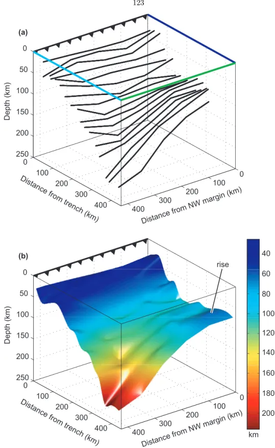
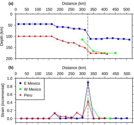
Slab Transition

The observed vertical oscillations or undulations of the plate surface are likely artificial and are the result of the 25 km wide gaps between the location of each seismicity fit. As such, the slab surface as shown in Figure 4.8b, with very little smoothing applied, is a more accurate representation of the data. An anomalous uplift in the NW corner (∼0–150 km from the NW margin) of the plate surface in the subduction region (∼325–450 km from the trench) should also be noted.

Figure 4.6: Map showing epicenters (stars) for earthquakes from the 1960–2013 ISC Bulletin event catalog as in Figure 4.5a

Ultra-slow Velocity Layer

Phase A is converted at the bottom of the USL and appears as a negative pulse at local stations. Shaded USL zones, possible USL and non-USL zones further explain our observations (Figure 4.10). The locations of the USL area and the approximate boundaries of the non-USL area are provided for reference.

Figure 4.8: 3D perspective view (looking west) of the transition from flat to normal subduction as constrained by seismicity

Discussion

This interpretation is consistent with the observed uplift of the Fitzcarrald arc in the Amazon foreland basin, which is attributed to the predicted continuation of the Nazca Ridge (Espurt et al., 2007). We propose that the initial subduction of the Nazca Ridge at 11◦S introduced additional water into the subduction zone as the slab dehydrated. Talc formation decreases wedge viscosity, which may facilitate plaque flattening (Manea and Gurnis, 2007; Kim et al., 2013).

Figure 4.16: 2D velocity models of the subduction zone structure along the PF (green squares) and PE (light blue squares) lines for the S56 ◦ E-oriented profile for event 20 (Figure 4.13, Table 4.2)

Conclusions

One possible explanation is that the reversal of the Cocos plate since the late Miocene (Ferrari et al., 2012) imposed stresses on the plate that resulted in tearing along pre-existing lines of weakness in the subducting plate located at flat-to-normal transitions . subduction (Dougherty and Clayton, 2014), where the plate was previously deformed. These lines of weakness include the predicted extension of the Orozco Fracture Zone to the west (Bandy et al., 2000; Dougherty et al., 2012;. The absence of a rupture in the slab along the Nazca Ridge or greater increase in slab dip is also confirmed with 2D waveform modeling.

Figure 4.18: Slab strain along the transition from flat to normal subduction in three regions

Supplemental Figures

Isacks (1976), Spatial distribution of earthquakes and subduction of the Nazca Plate beneath South America, Geology. Isacks (1979), Subduction of the Nazca plate beneath Peru: evidence from spatial distribution of earthquakes, Geophys. Clayton (2014), Structure of the subduction transition region from seismic array data in southern Peru, Geophys.

Figure 4.20: Perspective view (updip) of cross-sections of slab seismicity from the ISC (dots) and EHB (triangles) catalogs in trench-parallel bins h1 (top) to h18 (bottom; see Figure 4.6 for bin locations)

Abstract

Note: This chapter was written in 2009 and as a result the locations of non-volcanic earthquakes and slow slips may be out of date. Images and text will be updated to reflect any changes made during the preparation of this chapter for future publication.

Introduction

Eurasian plate

Data and Method
Results
Discussion and Conclusions
Future Work

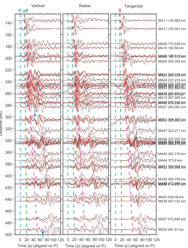
Teleseismic records from (left) stack data on six short-term arrays and from (right) broadband stations near the arrays, filtered to 0.5–1 Hz. The arrivals of the depth phases pP (blue box) and sP (green box), along with a possible reflection at the bottom of the Moho of the predominant plate (sMP; purple box) are also shown. Lateral variations in the amount of fluid released from the plate could account for the laterally heterogeneous structure of the proposed USL.