Chapter 11 Solution 1

(1)

Chapter 11, Solution 1.

) t 50 cos(

160 ) t (

v 

i(t) = –33sin(50t–30˚) = 33cos(50t–30˚+180˚–90˚) = 33cos(50t+60˚) p(t) = v(t)i(t) = 160x33cos(50t)cos(50t+60˚)

= 5280(1/2)[cos(100t+60˚)+cos(60˚)] = [1.320+2.640cos(100t+60˚)] kW.

P = [V_mI_m/2]cos(0–60˚) = 0.5x160x33x0.5 = 1.320 kW.

(2)

Using current division,

j1 Ω I2 I1

Vo

-j4 Ω 20^o A 5 Ω

1

1 4 6

5 1 4(2) 5 3

j j j

I j j j

 

 

  

2

5 1

5 1 4(2) 5 3

I 0

j j j

 

  

.

For the inductor and capacitor, the average power is zero. For the resistor,

2 2

1

1 1

| | (1.029) (5) 2.647 W

2 2

P I R 

5 1 2.6471 4.4118 Vo  I    j

1 * 1

( 2.6471 4.4118) 2 2.6471 4.4118

2 ^o 2

S  V I    j x    j

Hence the average power supplied by the current source is 2.647 W.

(3)

I

C 1600^˚ R

+ –

1 1₆ ₃

90 F 5.5556

j C 90 10 2 10 j

j x x x

 ^^  ^ ^ ^{ }

I = 160/60 = 2.667A

The average power delivered to the load is the same as the average power absorbed by the resistor which is

Pavg = 0.5|I|²60 = 213.4 W.

(4)

Using Fig. 11.36, design a problem to help other students better understand instantaneous and average power.

Although there are many ways to work this problem, this is an example based on the same kind of problem asked in the third edition.

Problem

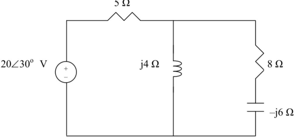
Find the average power dissipated by the resistances in the circuit of Fig. 11.36.

Additionally, verify the conservation of power. Note, we do not talk about rms values of voltages and currents until Section 11.4, all voltages and currents are peak values.

5 Ω

2030^o V j4 Ω 8 Ω

–j6 Ω

+ –

Figure 11.36 For Prob. 11.4.

Solution

We apply nodal analysis. At the main node, I1 5 Ω I2

Vo

2030^o V j4 Ω 8 Ω

–j6 Ω

+ –

(5)

20 30

5.152 10.639

5 4 8 6

o

o o o

o

V V V

V j

j j

      

 = 11.82164.16˚

For the 5-Ω resistor,

1

20 30

2.438 3.0661 A 5

o o o

I   V   

The average power dissipated by the resistor is

2 2

1 1 1

1 1

| | 2.438 5 14.86 W

2 2

P  I R  x x 

For the 8-Ω resistor,

I2 = Vo/(8–j6) = (11.812/10)(64.16+36.87)˚ = 1.1812101.03˚ A The average power dissipated by the resistor is

P2 = 0.5|I2|²R2 = 0.5(1.1812)²8 = 5.581 W The complex power supplied is

S = 0.5(Vs)(I1)^* = 0.5(2030˚)(2.4383.07˚) = 24.3833.07˚

= (20.43+13.303) VA

Adding P1 and P2 gives the real part of S, showing the conservation of power.

P = 14.86+5.581 = 20.44 W which checks nicely.

(6)

Converting the circuit into the frequency domain, we get:

1  2 

W 4159 . 1 2 1

6828 . P 1

38 . 25 6828 . 1 2 j 2 6 j

) 2 j 2 ( 6 1 j

40 I 8

2 1

1













 







 



P_1Ω = 1.4159 W P3H = P0.25F = 0 W

W 097 . 5 2 2

258 . P 2

258 . 2 38 . 25 6828 . 21 j 2 6 j

6 I j

2 2

2







 

 



P_2Ω = 5.097 W

j6 –j2

+

8–40˚ _

(7)

3 3

20 mH  j L  j10 x20 10x ^  j20 25

j 10

x 40 x 10 j

1 C

j F 1

40  3 6 

 

 _

We apply nodal analysis to the circuit below.

V_o 20I_x

+ – I_x

j20 50

60o

–j25 10

25 0 j 50

0 V 20 j 10

I 20

6 V^o ^x ^o 



 

 

 But

25 j 50 I_x V^o

  . Substituting this and solving for V_o leads



⁰^.⁰² ^j⁰^.⁰⁴ ⁰^.⁰¹²⁸⁰² ^j⁰^.⁰⁰⁹⁵⁹⁸ ⁰^.⁰¹⁶ ^j⁰^.⁰⁰⁸



^V ⁶

6 57 V

. 26 9 . 55

1 )

57 . 26 9 . 55 )(

43 . 63 36 . 22 (

20 43

. 63 36 . 22

1

6 25 V

j 50

1 )

25 j 50 (

1 ) 20 j 10 (

20 20

j 10

1

o

o o







 

 







 









 





 

 



 



 



(0.0232 – j0.0224)V_o = 6 or V_o = 6/(0.03225–43.99˚) = 186.0543.99˚ volts.

|Ix| = 186.05/55.9 = 3.328

We can now calculate the average power absorbed by the 50-Ω resistor.

P_avg = [(3.328)²/2]x50 = 276.8 W.

(8)

Applying KVL to the left-hand side of the circuit,

o o 0.1 4

20

8  I  V (1)

Applying KCL to the right side of the circuit, 5 0

j 10 5

8 _o  Vj¹  V¹  I

But, _o ₁ ₁ _o

10 5 j 10 5

j 10

10 V V V

V     

Hence, 0

10 50

j 5 j

8 _o 10 _o  V^o  V

I

o o j0.025V

I  (2)

Substituting (2) into (1),

) j 1 ( 1 . 0 20

8  V_o  j

1 20 80

o   

V







 -25

2 8 10

1 o

I V

 



 







 





 (10)

2 64 2 R 1 2

P 1 I₁ ² 160W

(9)

We apply nodal analysis to the following circuit.

At node 1,

20 j - 10

6 jV¹ V¹V² V1  j120V2 (1) At node 2,

5 40 .

0 _o _o V² I I   But,

j20 -

2 1 o

V

I V 

 Hence,

40 j20

-

) (

5 .

1 V₁ V₂ V₂

 

2 1 (3 j)

3V   V (2)

0 j 3 3 360

j  V₂  V₂  V₂  j6) -1 37 ( 360 j 6

360 j

2    

V

j6) -1 37(

9 40

2

2  V  

I

 



 



 

 (40)

37 9 2 R 1 2

P 1

2 2

I2 43.78W

40 

j10  0.5 I_o

60 A

V1 I_o -j20  V2

I₂

(10)

This is a non-inverting op amp circuit. At the output of the op amp,

3 2

3 1

(10 6) 10

1 1 (8.66 5) 20.712 28.124

(2 4) 10

o s

Z j x

V V j j

Z j x

    

          The current through the 20-k resistor is

0.1411 1.491 mA

20 12

o o

I V

k j k

  

 j or |Io| = 1.4975 A

P = [|Io|²/2]R = [1.4875²/2]10^–6x20x10³

= 22.42 mW

(11)

No current flows through each of the resistors. Hence, for each resistor, . It should be noted that the input voltage will appear at the output of each of the op amps.



P 0W

(12)

, ,

377

 R10⁴ C20010^-9 754 . 0 ) 10 200 )(

10 )(

377 (

RC ⁴  ^-9 







RC) 37.02 (

tan^-1











 

 -37.02 7.985 -37.02 k

) 754 . 0 ( 1

k Z 10

ab 2

mA t

t t

i( )33sin(377 22)33cos(377 68) I = 33–68˚ mA

 

2

10 ) 37.02 - 985 . 7 ( 10 33 2

2 3 3

2    

 I Z x ^

S ^ab

S = 4.348–37.02˚ VA



 S cos(37.02)

P 3.472 W

(13)

We find the Thevenin impedance using the circuit below.

j2 Ω

4 Ω -j3 Ω

5 Ω

We note that the inductor is in parallel with the 5-Ω resistor and the combination is in series with the capacitor. That whole combination is in parallel with the 4-Ω resistor. Thus,













 

 



 







 





39 . 46 1936 . 1

22 . 15 86 . 4

) 61 . 61 4502 . 1 ( 4 2758

. 1 j 69 . 4

) 2758 . 1 j 6896 . 0 ( 4 2 j 5

2 xj 3 5 j 4

2 j 5

2 xj 3 5 j 4 Z_Thev

ZThev = 0.8233 – j0.8642 or ZL = [823.3 + j864.2] mΩ. We obtain V_Th using the circuit below. We apply nodal analysis.

2j Ω

I

4 Ω –j3 Ω V₂ +

1650^o V

V_Th 5 Ω –

+ –

(14)

165 ) 17 . 67 4123 . 0 ( ) 55 . 46 5235 . 0 (

165 ) 5 . 0 12 . 0 16 . 0 ( ) 2 . 0 5 . 0 12 . 0 16 . 0 (

5 0 0 2

165 3

4 165

2 2 2 2

2



























 

 



V

j j

V j

j

V j

V j V

4.125

Thus, V2 = 129.94–20.62˚V = 121.62–j45.76

I = (165 – V₂)/(4 – j3) = (165 – 121.62 + j45.76)/(4 – j3)

= (63.0646.52˚)/(5–36.87˚) = 12.61383.39˚ = 1.4519+j12.529 VThev = 165 – 4I = 165 – 5.808 – j50.12 = [159.19 – j50.12] V = 166.89–17.48˚V

We can check our value of V_Thev by letting V₁ = V_Thev. Now we can use nodal analysis to solve for V1.

At node 1,

25 . 41 )

3333 . 0 2 . 0 ( ) 3333 . 0 25 . 0 ( 5 0

0 3

4 165

2 1

2 2 1

1        



  V j V j V

j V V V

At node 2,

5 . 82 )

1667 . 0 ( 3333 . 0 2 0

165

3 ¹ ²

2 1

2 j V j V j

j V j

V

V       



>> Y=[(0.25+0.3333i),-0.3333i;-0.3333i,(0.2-0.1667i)]

Y =

0.2500 + 0.3333i 0 - 0.3333i 0 - 0.3333i 0.2000 - 0.1667i

>> I=[41.25;–82.5i]

I =

41.2500 0 -20.0000i

>> V=inv(Y)*I V =

(15)

159.2221 – 50.1018i 121.6421–45.7677i

Please note, these values check with the ones obtained above.

To calculate the maximum power to the load, |IL| = (166.89/(2x0.8233)) = 101.34 A

P_avg = [(|I_L|_rms)²0.8233]/2 = 4.228 mW.

(16)

For maximum power transfer to the load, ZL = [120 – j60] Ω. IL = 165/(240) = 0.6875 A

P_avg = [|I_L|²120]/2 = 28.36 W.

(17)

Using Fig. 11.45, design a problem to help other students better understand maximum average power transfer.

Problem

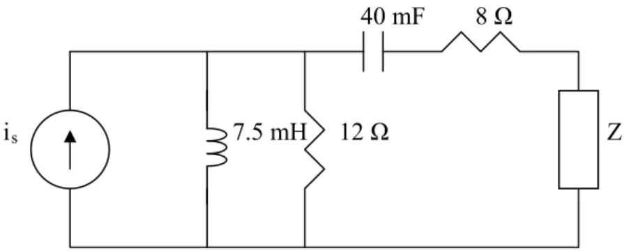
It is desired to transfer maximum power to the load Z in the circuit of Fig. 11.45. Find Z and the maximum power. Let i_s 5 cos 40t A.

40 mF 8 Ω

i_s 7.5 mH 12 Ω Z

Figure 11.45 For Prob. 11.14.

Solution

We find the Thevenin equivalent at the terminals of Z.

40 mF 1 1 ₃

0.625 40 40 10 j j C j x x ^

  

7.5 mH  j L  j40 7.5 10x x ^³  j0.3 To find ZTh, consider the circuit below.

-j0.625 8 Ω

j0.3 12 Ω Z_Th

(18)

12 0.3

Z_L = (Z_Thev)^* = [8.008 + j0.3252] Ω. Z_L = (Z_Thev)^* = [8.008 + j0.3252] Ω.

To find VTh, consider the circuit below.

-j0.625 8 Ω

I₁ +

50^o j0.3 12 Ω VTh

50 j0.3 12 ^o Ω VTh

– –

By current division, By current division,

I1 = 5(j0.3)/(12+j0.3) = 1.590˚/12.0041.43˚ = 0.1249688.57˚ I1 = 5(j0.3)/(12+j0.3) = 1.590˚/12.0041.43˚ = 0.1249688.57˚

= 0.003118 + j0.12492A = 0.003118 + j0.12492A

VThev rms = 12I1/

VThev rms = 12I1/ 2 = 1.060388.57˚V

I_Lrms = 1.060388.57˚/2(8.008) = 66.288.57˚mA Pavg = |ILrms|²8.008 = 35.09 mW.

(19)

To find Z_eq, insert a 1-A current source at the load terminals as shown in Fig. (a).

At node 1,

2 o o

2 o

o j

j - j

1 V V V V V

V   



 (1)

At node 2,

o 2

o 1 j (2 j)

j 2 -

1 V V V V

V     



 (2)

2 2

2 (2 j)(j) (1 j) j

1 V   V   V

j 1

1

2  

V

5 . 0 5 . 2 0 1 1

2 j j

eq  V    

Z



 ^*eq

L Z

Z [0.5 j0.5] We now obtain V_Thev from Fig. (b).

1 0

2  12 

 j

o o

o

V V V

1 A

1  1 2 -j 

j  2 V_o

+ Vo



(a)

1  -j 

j  2 V_o

+ Vo



(b) 120 V

+ +

VThev

 

(20)

j 1

–V_o (-j2V_o)V_Th 0 j

j

Thev     

1

) 2 1 )(

12 j2) (

- (1 V_o V



² ⁰^.⁵



⁰^.⁵

2 2

5 12 5 . 2 0

5 . 0 5 . 0 5 . 0 5 . 0

2 2 2

max x

j j

V P

Thev 



 

 







 

= 90 W

(21)

20 5 / 1 4

1 F 1

20 / 1 , 4 H

1 ,

4 j

x j C j j

L

j    





  



We find the Thevenin equivalent at the terminals of ZL. To find VThev, we use the circuit shown below.

0.5V_o

2 V1 4 V2

+ + +

10<0o

Vo -j5 j4 VThev

- -

- At node 1,

2 2 1

1 1 1

1 5 V (1.25 j0.2) 0.25V

4 V V V

5 . 5 0 j V 2

V

10       

 

 (1)

At node 2,

) 25 . 0 25 . 0 ( 5

. 0 4 0

25 .

4 0 ¹ ²

2 1 2

1 V V j

j V V V

V        

(2) Solving (1) and (2) leads to

o

Thev V j

V  ₂ 6.1947 7.07969.407248.81

(22)

0.5V₁

2 V₁ 4 V₂

-j5 j4

1A

At node 1,

2 1

2 1 1 1

1 0 0 (1 0.2) 0.25

25 4 . 5 0

2 V V V j V

j V V

V        

 (3)

At node 2,

) 25 . 0 25 . 0 ( 5

. 0 4 1

25 . 4 0

1 ¹ ² ₁ ² V₁ V₂ j

j V V V

V         

 (4)

Solving (1) and (2) gives

o

eq V j

Z 1.9115 3.3274 3.837 60.12 1

2    

 and Z_L = 3.837–60.12° Ω



 

 2 4 1.9115

4072 . 9115 9 . 1 2

|

| ²

2 2

max Z Z x x

P V

L eq

Th 5.787 W

(23)

We find Z_eq at terminals a-b following Fig. (a).

   

10 70

) 20 40 )(

10 30 40 ( 20

||

30

10 j

j j j

eq j

 

 







Z = 20 Ω = ZL

We obtain V_Thev from Fig. (b).

Using current division,

3 . 2 j 1 . 1 - ) 5 j 10( j 70

20 j 30

1    

I

7 . 2 j 1 . 1 ) 5 j 10( j 70

10 j 40

2    

I

70 j 10 10

j

30 ₂ ₁

Th  I  I  

V



^



^ ^

 20

) 20 2 )(

2 (

5000

2 ² ²

2

max Z x

Z Z

P _L

L eq

VTh

31.25 W

-j10  30 

40  j20 

(a)

a b

I1 I2

-j10  30 

j5 A + V^Thev 

j20  40 

(b)

(24)

We find Z_Th at terminals a-b as shown in the figure below.

j10 80 (80)(-j10) 20

j30 -j10) (

||

80 40

||

40

30     

 j ZTh

154 . 20 23 .

21 j

Th  

Z



 ^*Th

L Z

Z [21.23–j20.15] Ω

40  -j10 

80  40 

a Z^th j30 

b

(25)

At the load terminals,

j 9

j) (6)(3 -j2

) j 3 (

||

6 2 j

Th -









 Z

561 . 1 j 049 .

Th 2 

Z



 Th

RL Z 2.576 Ω

To get V_Th, let Z6||(3j)2.049 j0.439. By transforming the current sources, we obtain

487 . 14 62 . 67 ) 0 33

( j

Th    Z 

V = 69.1612.09˚

Pmax =

2 576 . 2 576 . 2 561 . 1 049 . 2

16 .

69 ²



 j = 258.5 W.

(26)

Combine j20  and -j10  to get j20||-j10-j20.

To find Z_Th, insert a 1-A current source at the terminals of R_L, as shown in Fig. (a).

At the supernode,

10 j - 20 j -

1 40V¹ V¹ V²





2 1 j4 )

2 j 1 (

40  V  V (1)

Also, V₁ V₂ 4 I_o, where

40 - ₁

o

I  V

1 . 1 1

.

1 ₁ ₂ ₁ V²

V V

V    (2)

2

2 j4

1 . ) 1 2 j 1 (

40 V V



 

 



4 . 6 j 1

44

2  

V







 1.05 j6.71 1

2 Th

Z V



 Th

RL Z 6.792

1 A 40 

-j10 

V₁ V₂

(a) 4 I_o Io

+  -j20 

(27)

To find V_Th, consider the circuit in Fig. (b).

At the supernode,

j10 - j20 - 40

165 V₁ V₁ V₂



 

2

1 4

) 2 1 (

165  j V  j V (3)

Also, V₁ V₂ 4 I_o, where

40 165 V₁ Io   1

. 1

5 .

2 16

1

 V 

V (4)

150–j30(0.9091 j5.818)V₂







 

 

 



 

 25.98 92.43

12 . 81 889 . 5

31 . 11 97 . 152 818 . 5 9091 . 0

30 150

2 j

j

Th V

V P_max =

2 792 . 6 792 . 6 71 . 6 05 . 1

98 .

25 ²



 j = 21.51 W

40 

-j10 

V1 V2

(b) 4 Io

I_o

+  -j20 

+ Vth

 1650 V ⁺



(28)

We find Z_Th at terminals a-b, as shown in the figure below.

] ) 30 j 40 (

||

100 10 j - [

||

Th 50  

Z

where 31.707 j14.634

30 j 140

) 30 j 40 )(

100 ) (

30 j 40 (

||

100      

634 . 4 j 707 . 81

) 634 . 4 j 707 . 31 )(

50 ) ( 634 . 4 j 707 . 31 (

||

Th 50   

Z

73 . 1 j 5 .

Th 19 

Z



 Th

RL Z 19.58

50  100  -j10 

a 40 

Z_th j30 

b

(29)

i(t) = [2–2cos(2t)] amps

(30)

Using Fig. 11.54, design a problem to help other students to better understand how to find the rms value of a waveshape.

Problem

Determine the rms value of the voltage shown in Fig. 11.54.

v(t) (V) 10

0 1 2 3 4 t (s) Figure 11.54 For Prob. 11.23.

Solution

1

2 2 2

0 0

1 1 100

( ) 10

3 3

T

Vrms v t dt dt

T









V_rms = 5.7735 V

(31)

, 2 T







 

2 t 1 5, -

1 t 0 , ) 5 t ( v



⁵ ^dt ⁽^-5) ^dt



²⁵₂ ^[¹ ¹^] ²⁵

2

V 1 ²

1 1 2

0 2 2

rms 







  

 Vrms 5V

(32)

 

266 . 3 3 f 32

3 ] 32 16 0 16 3[ 1

dt 4 dt 0 dt ) 4 3 ( dt 1 ) t ( T f

f 1

rms

3 2 2 2

1 1

0 T 2

0 2 rms2













   

frms = 3.266

(33)

,

4 T







 

4 t 2 20

2 0 ) 5

( t

t v

250 ] 800 200 4[ ) 1

20 ( 4 10

1 ⁴

2 2 2

0 2

2   

 





^dt



^dt

V_rms



Vrms 15.811 V.

(34)

, 5

T i(t)t, 0t5

333 . 15 8 125 3

t 5 dt 1 5 t

I 1 ⁵₀

5 3 0

2 2

rms 



   



Irms 2.887A

(35)

 ^

^

^ 

 ₀² ² ₂⁵ ²

2

rms (4t) dt 0 dt

5 V 1

533 . 8 ) 8 15( 16 3

t 16 5

V 1 ²₀

3 2

rms    



Vrms 2.92V



 2

533 . 8 R P V

2

rms 4.267W

(36)

, 20 T











 

25 t 15 6t 120 -

15 5

6 ) 60

( t t

t i



   





⁵¹⁵ ²



¹⁵²⁵ ²

2 (60 6 ) (-120 6t)

20

1 t dt dt

I_eff



     





⁵¹⁵ ²



¹⁵²⁵ ²

2 (900 180 9 ) (9t 360t 3600)

5

1 t t dt dt

I_eff

   



² ³ ¹⁵⁵ ³ ² ¹⁵²⁵



2 900 90 3 3 180 3600

5

1 t t t t t t

I_eff      

300 ] 750 750 5[

2 1  

Ieff



Ieff 17.321 A



I R

P ²_eff (17.321)²x12 = 3.6 kW.

(37)







 

4 t 2 1 -

2 t 0 ) t

t ( v



^t ^dt ⁽^-1) ^dt



₄¹ ₃⁸ ² ¹^.¹⁶⁶⁷

4

V 1 ⁴

2 2 2

0 2 2

rms 

 







 



Vrms 1.08V

(38)

6667 . 8 3 16

4 2 ) 1

4 ( )

2 2 ( ) 1 2 ( 1²

0

1

0

2

1 2 2

2 

 





 



  





^v ^t ^dt



^t ^dt



^dt

V rms

V 944 .

2 Vrms

(39)



 





⁰¹ ² ²



¹²

2

rms (10t ) dt 0dt

2 I 1

5 10 50 t dt t 50

I ¹₀

1 5 0

4 2

rms 



  



Irms 3.162A

(40)

3 4

2 2 1 2 2

0

0 1 3

1 1

( ) 25 25 ( 5 20)

6

T

Irms i t dt t dt dt t dt

T

 

       

 

   

3 3

2 1 1 2 4

25 25(3 1) (25 100 400 ) 11.1056

0 3

6 3 3

rms

t t

I  t 

       

 t 

I_rms = 3.332 A

(41)

472 . 4 20

20 3 36

9 3 1

6 )

3 3 ( ) 1 1 (

2

0 3

3 2 2 2

0 2 0

2 2













 





 



  

rms

T rms

f t

dt dt

t dt

t T f

f

frms = 4.472

(42)

 ^

^

^

^

^

^

^

^

^ 

 ₀¹ ² ₁² ² ₂⁴ ² ₄⁵ ² ₅⁶ ²

2

rms 10 dt 20 dt 30 dt 20 dt 10 dt

6 V 1

67 . 466 ] 100 400 1800 400 100 6[

V_rms²  1     



Vrms 21.6V

(43)

(a) I_rms = 10 A

(b) 2

16 9 2

4 3

2 2

2     





 rms

rms V

V 4.528V (checked)

(c) 9.055 A

2 64 36 

 Irms

(d) 4.528V

2 16 2

25 

 Vrms

(44)

Design a problem to help other students to better understand how to determine the rms value of the sum of multiple currents.

Problem

Calculate the rms value of the sum of these three currents:

i1 = 8, i2 = 4 sin(t + 10), i3 = 6 cos(2t + 30) A Solution

) 30 2 cos(

6 ) 10 sin(

4

3 8

2 1

o

o t

t i

i i

i       

A 487 . 9 2 90

36 2 64 16

3 2 2

2 1

2       

 ^rms ^rms ^rms

rms I I I

I

(45)

2 2

1 *

1

220 390.32 124

S V

 Z  

2 2

2 *

2

220 944.4 1180.5

20 25

S V j

Z j

   



2 2

3 *

3

220 300 267.03

90 80

S V j

Z j

   



S    S₁ S₂ S₃ 1634.7 j913.471872.6 29.196 VA^o (a) P = Re(S) = 1634.7 W

(b) Q = Im (S) = 913.47 VA (leading) (c ) pf = cos (29.196^o) = 0.8732

(46)

(a) ZL = 4.2 + j3.6 = 5.5317 40.6^o pf = cos 40.6 = 0.7592

2 2

*

220 6.643 5.694 kVA

5.5317 40.6

rms

o

S V j

 Z   

  P = 6.643 kW Q = 5.695 kVAR (b)

3

1 2

2 2

(tan tan ) 6.643 10 (tan 40.6 tan 0 )

312 F 2 60 220

o o

rms

P x

C V x x

  

 ^  ^

   ,

{It is important to note that this capacitor will see a peak voltage of 220 2 = 311.08V, this means that the specifications on the capacitor must be at least this or greater!}

(47)

Design a problem to help other students to better understand apparent power and power factor.

Problem

A load consisting of induction motors is drawing 80 kW from a 220-V, 60 Hz power line at a pf of 0.72 lagging. Find the capacitance of a capacitor required to raise the pf to 0.92.

Solution

0 1 1

1 0.72 cos 43.94

pf      

0

2 2

2 0.92 cos 23.07

pf      

3

1 2

2 2

(tan tan ) 80 10 (0.9637 0.4259)

2.4 mF 2 60 (220)

rms

P x

C V x x

 

 ^  ^

   ,

{Again, we need to note that this capacitor will be exposed to a peak voltage of 311.08V and must be rated to at least this level, preferably higher!}

(48)

(a) -j6 j

(-j2)(-j3) -j3

||

-j2 ) 2 j 5 j (

||

2 j

-    









4 j6 7.211 -56.31 ZT





cos(-56.31 )

pf 0.5547 (leading)

(b) 0.64 j1.52

3 j 4

) j 4 )(

2 j ) ( j 4 (

||

2

j      





 

 





 0.4793 21.5

44 . 0 j 64 . 1

44 . 0 j 64 . ) 0 j 52 . 1 j 64 . 0 (

||

1 Z





cos(21.5 )

pf 0.9304 (lagging)

(49)

(a) S=120, pf 0.707cos   45^o

cos sin 84.84 84.84 VA

S S   jS    j

(b) 120

1.091 A rms

rms rms rms 110

rms

S V I I S

  V  

(c) _rms² ₂ 71.278 71.278

rms

S I Z Z S j

   I   

(d) If Z = R + jL, then R = 71.278 Ω

71.278

2 71.278 0.1891 H

2 60

L fL L

 ^  ^ ^^ ^ x ^ = 189.1 mH.

(50)

Design a problem to help other students to better understand complex power.

Problem

The voltage applied to a 10-ohm resistor is v(t) = 5 + 3 cos(t + 10) + cos(2t + 30) V (a) Calculate the rms value of the voltage.

(b) Determine the average power dissipated in the resistor.

Solution

(a) 30 5.477V

2 1 2 25 9

3 2 2

2 1

2       

 ^rms ^rms ^rms

rms V V V

V

(b) 30/10 3 W

2  

 R P V ^rms

(51)

6

1 1

40 12.5

2000 40 10

F j

j C j x x

 ^^  ^ ^ ^{ }

60mH  j L  j2000 60 10x x ^3  j120 We apply nodal analysis to the circuit shown below.

100 4

30 12.5 20 120

o x o

V I V V_o

j j

   

 But

120

o x

I V

 j . Solving for V_o leads to 2.9563 1.126

Vo   j

I_o 30 Ω -j12.5 20 Ω Vo

Ix

1000^o ₊ j120 + 4I_x

–

100 2.7696 1.1165

30 12.5

o o

I V j

j

   



1 * 1

(100)(2.7696 .1165) 138.48 55.825 VA 2 ^{s o} 2

S  V I   j   j

S = (138.48 – j55.82) VA

(52)

(a) 2200 46.9V 2

20 60

2 2

2rms     Vrms 

V

A

I_rms 1.125 1.061

2 5 . 1 0

2

2   



(b) p(t) = v(t)i(t) = 20 + 60cos100t – 10sin100t – 30(sin100t)(cos100t); clearly the average power = 20W.

(53)

(a) SVI^* (22030)(0.5-60)110-30



S [95.26 j55]VA Apparent power =110VA Real power =95.26W Reactive power =55VAR

pf is leading because current leads voltage (b) SVI^*  (250-10)(6.225)155015



S [497.2 j401.2]VA Apparent power =1550VA Real power =1497.2W Reactive power =401.2VAR

pf is lagging because current lags voltage (c) SVI^* (1200)(2.415)28815



S [278.2 j74.54]VA Apparent power =288VA Real power =278.2W

Reactive power =74.54VAR

pf is lagging because current lags voltage (d) SVI^* (16045)(8.5-90)1360-45



S [961.7 – j961.7] VA Apparent power =1360VA Real power = 961.7 W Reactive power =-961.7VAR

pf is leading because current leads voltage

(54)

(a) V_112_10_, I4-50_









 224 60

2

1 _*

I V

S [112 j194]VA

Average power =112W Reactive power =194VAR (b) V_160_0_, I445_









 320 -45 2

1 _*

I V

S 226.3 – j226.3

Average power = 226.3 W Reactive power = –226.3 VAR

(c)    12830

30 - 50

) 80

( ²

* 2

Z

S V 110.85 + j64

Average power = 110.85 W Reactive power = 64VAR

(d) S I ²Z(100)(10045)[7.071 j7.071]kVA Average power =7.071kW

Reactive power =7.071kVAR

(55)

(a) SP jQ[269 j150]VA (b) pf cos0.9  25.84

31 . ) 4588 84 . 25 sin(

2000 sin

S Q sin

S

Q       

48 . 4129 cos

S P 



S [4.129 j ]2 kVA

(c) 0.75

600 450 S sin Q sin

S

Q     

59 .

48

 , pf 0.6614 86 . 396 ) 6614 . 0 )(

600 ( cos S

P  



S [396.9 j450]VA

(d) 1210

40 ) 220 S (

2 2



 Z V

8264 . 1210 0 1000 S

cos P cos

S

P     





 34.26

25 . 681 sin

S

Q 



S [1 j0.6812]kVA

(56)

(a) sin(cos (0.86))kVA 86

. 0 j 4

4 ^-¹

 S



S [4 j2.373]kVA

(b) 0.8 cos sin 0.6

2 6 . 1 S

pf  P     







1.6 j2sin

S [1.6 j1.2]kVA (c) SV_rmsI^*_rms (20820)(6.550)VA







1.352 70

S [0.4624 j1.2705]kVA

(d)      

56.31 - 11 . 72

14400 60

j 40

) 120

( ²

* 2

Z S V







199.7 56.31

S [110.77 j166.16]VA

(57)

(a) sin(cos (0.8))

8 . 0 j1000 1000

jQ

P   ^-¹

 S

750 j 1000

 S

But, _*

2 rms

Z S V

23 . 23 j 98 . 750 30 j 1000

) 220

( ²

2

*  rms    

S Z V



Z [30.98 j23.23] (b) S I_rms ²Z

 



 2 2

rms (12)

2000 j 1500 I

Z S [10.42 j13.89]

(c) _ _ _



 



 1.6 -60

) 60 4500 )(

2 (

) 120 ( 2

2 2 2

* rms

S V S

Z V







1.6 60

Z [0.8 j1.386]

(58)

(a) Z_T 2(10j5)||(8j6)

j 18

20 j 2 110 j

18

) 6 j 8 )(

5 j 10 2 (

T        

Z









8.152 j0.768 8.188 5.382 ZT





cos(5.382 )

pf 0.9956 (lagging)

(b) (8.188 -5.382 )

) 16 ( ²

* 2

*



 



 Z

I V V S





31.26 5.382 S





Scos

P 31.12 W

(c) QSsin2.932 VAR (d) S S 31.26 VA

(e) S_31.26_5.382__ (31.12+j2.932) VA

(a) 0.9956 (lagging, (b) 31.12 W, (c) 2.932 VAR, (d) 31.26 VA, (e) [31.12+j2.932]

VA

(59)

749 j 4200 S

S S S

500 j 1000 S

2749 j 1200 9165

. 0 x 3000 j 4 . 0 x 3000 S

1500 j 2000 6

. 8 0 . 0 j2000 2000

S

C B A C B A





























(a) _

 ₂  ₂

749 4200

pf 4200 0.9845 leading

(b)   











 ^ ^ 35.55 55.11

45 120

749 j I 4200

I V

S _rms _rms _rms

Irms = 35.5555.11˚ A.

(60)

S = SA + SB + SC = 4000(0.8–j0.6) + 2400(0.6+j0.8) + 1000 + j500 = 5640 + j20 = 56400.2˚

(a)

A I

V S V

S S V I S

rms rms

C A rms

B rms



















 

 



 



 

8 . 29 47 8 . 29 47

8 . 29 30 47

120 2 . 0 5640

(b) pf = cos(0.2˚) ≈ 1.0 lagging.

(61)

Consider the circuit shown below.





  

  1.6 16.87 3

j 4

20 - 8 I1







  1.6 -110 5

j 20 - 8 I2

) 4643 . 0 j 531 . 1 ( ) 504 . 1 j -0.5472

2 (

1    

I I I









0.9839 j1.04 1.432 -46.58 I

For the source,

) 46.58 432

. 1 )(

20 - 8

* (    

VI S







11.456 26.58

S (10.24+j3.12) VA

For the capacitor,



 I₁ ²Z_c (1.6)²(-j3)

S –j7.68 VA

For the resistor,



 I₁ ²Z_R (1.6)²(4)

S 10.24 VA

For the inductor,



 I₂ ²Z_L (1.6)²(j5)

S j12.8 VA

(62)

Using Fig. 11.74, design a problem to help other students to better understand the conservation of AC power.

Problem

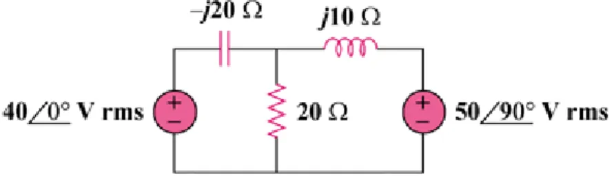
Find the complex power absorbed by each of the five elements in the circuit of Fig.

11.74.

Figure 11.74 Solution

We apply mesh analysis to the following circuit.

For mesh 1,

2 1 20I I

) 20 j 20 (

40  

2

1 I

I ) j 1 (

2   (1)

For mesh 2,

1

2 20I

I ) 10 j 20 ( 50 j

-   

2 1 (2 j)I I

-2 j5

-    (2)

Putting (1) and (2) in matrix form,











 





2 1

I I j 2 2 -

1 - j 1 j5 -

2

5090 V rms 400 V rms

j10  -j20 

I3

20  ⁺_

+  I₁ I₂

(63)

j 1



 , ₁ 4 j3, ₂ -1 j5









 

 



  (7 j) 3.535 8.13 2

1 j 1

3 j I₁ ¹ 4









 

 



  2 j3 3.605 -56.31

j 1

5 j 1 I₂ ² -



















I I (3.5 j0.5) (2 j3) 1.5 j3.5 3.808 66.8 I₃ ₁ ₂

For the 40-V source,



 

  



 (7 j)

2 ) 1 40 ( - -VI₁^*

S [-140j20]VA

For the capacitor,



 c

2

1 Z

I

S -j250VA

For the resistor,



 I₃ ² R

S 290VA

For the inductor,



 L

2

2 Z

I

S j130VA

A For the j50-V source,







VI^*₂ (j50)(2 j3)

S [-150 j100]V

Chapter 11 Solution 1





 





   

















 

   







 

 









   









 













   

  

 







 

 ^

^ 

 ^

^

^

^

^ 