Chapter 3
Geometric Representations and Transformations
This chapter provides important background material that will be needed for Part II. Formulating and solving motion planning problems require defining and manip- ulating complicated geometric models of a system of bodies in space. Section 3.1 introduces geometric modeling, which focuses mainly on semi-algebraic modeling because it is an important part of Chapter 6. If your interest is mainly in Chapter 5, then understanding semi-algebraic models is not critical. Sections 3.2 and 3.3 describe how to transform a single body and a chain of bodies, respectively. This will enable the robot to “move.” These sections are essential for understanding all of Part II and many sections beyond. It is expected that many readers will al- ready have some or all of this background (especially Section 3.2, but it is included for completeness). Section 3.4 extends the framework for transforming chains of bodies to transforming trees of bodies, which allows modeling of complicated sys- tems, such as humanoid robots and flexible organic molecules. Finally, Section 3.5 briefly covers transformations that do not assume each body is rigid.
3.1 Geometric Modeling
A wide variety of approaches and techniques for geometric modeling exist, and the particular choice usually depends on the application and the difficulty of the problem. In most cases, there are generally two alternatives: 1) aboundary repre- sentation, and 2) a solid representation. Suppose we would like to define a model of a planet. Using a boundary representation, we might write the equation of a sphere that roughly coincides with the planet’s surface. Using a solid representa- tion, we would describe the set of all points that are contained in the sphere. Both alternatives will be considered in this section.
The first step is to define theworldW for which there are two possible choices:
1) a 2D world, in which W = R2, and 2) a 3D world, in which W = R3. These choices should be sufficient for most problems; however, one might also want to allow more complicated worlds, such as the surface of a sphere or even a higher
81
dimensional space. Such generalities are avoided in this book because their current applications are limited. Unless otherwise stated, the world generally contains two kinds of entities:
1. Obstacles: Portions of the world that are “permanently” occupied, for example, as in the walls of a building.
2. Robots: Bodies that are modeled geometrically and are controllable via a motion plan.
Based on the terminology, one obvious application is to model a robot that moves around in a building; however, many other possibilities exist. For example, the robot could be a flexible molecule, and the obstacles could be a folded protein.
As another example, the robot could be a virtual human in a graphical simulation that involves obstacles (imagine the family of Doom-like video games).
This section presents a method for systematically constructing representations of obstacles and robots using a collection of primitives. Both obstacles and robots will be considered as (closed) subsets of W. Let theobstacle region O denote the set of all points in W that lie in one or more obstacles; hence, O ⊆ W. The next step is to define a systematic way of representingO that has great expressive power while being computationally efficient. Robots will be defined in a similar way; however, this will be deferred until Section 3.2, where transformations of geometric bodies are defined.
3.1.1 Polygonal and Polyhedral Models
In this and the next subsection, a solid representation of O will be developed in terms of a combination ofprimitives. Each primitive Hi represents a subset of W that is easy to represent and manipulate in a computer. A complicated obstacle region will be represented by taking finite, Boolean combinations of primitives.
Using set theory, this implies that O can also be defined in terms of a finite number of unions, intersections, and set differences of primitives.
Convex polygons First consider O for the case in which the obstacle region is a convex, polygonal subset of a 2D world, W = R2. A subset X ⊂ Rn is called convexif and only if, for any pair of points in X, all points along the line segment that connects them are contained in X. More precisely, this means that for any x1, x2 ∈X and λ∈[0,1],
λx1+ (1−λ)x2 ∈X. (3.1)
Thus, interpolation between x1 and x2 always yields points in X. Intuitively, X contains no pockets or indentations. A set that is not convex is called nonconvex (as opposed toconcave, which seems better suited for lenses).
A boundary representation ofO is anm-sided polygon, which can be described using two kinds of features: vertices and edges. Every vertex corresponds to a
“corner” of the polygon, and every edge corresponds to a line segment between a
3.1. GEOMETRIC MODELING 83
Figure 3.1: A convex polygonal region can be identified by the intersection of half-planes.
pair of vertices. The polygon can be specified by a sequence, (x1, y1), (x2, y2),. . ., (xm, ym), ofm points in R2, given in counterclockwise order.
A solid representation of O can be expressed as the intersection of m half- planes. Each half-plane corresponds to the set of all points that lie to one side of a line that is common to a polygon edge. Figure 3.1 shows an example of an octagon that is represented as the intersection of eight half-planes.
An edge of the polygon is specified by two points, such as (x1, y1) and (x2, y2).
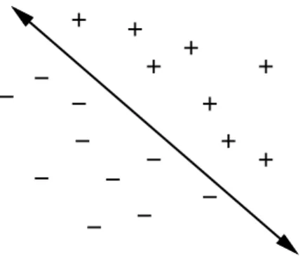
Consider the equation of a line that passes through (x1, y1) and (x2, y2). An equation can be determined of the form ax +by+c = 0, in which a, b, c ∈ R are constants that are determined from x1, y1, x2, and y2. Let f : R2 → R be the function given by f(x, y) = ax+by+c. Note that f(x, y) < 0 on one side of the line, and f(x, y) > 0 on the other. (In fact, f may be interpreted as a signed Euclidean distance from (x, y) to the line.) The sign of f(x, y) indicates a half-plane that is bounded by the line, as depicted in Figure 3.2. Without loss of generality, assume that f(x, y) is defined so that f(x, y) <0 for all points to the left of the edge from (x1, y1) to (x2, y2) (if it is not, then multiply f(x, y) by −1).
Let fi(x, y) denote the f function derived from the line that corresponds to the edge from (xi, yi) to (xi+1, yi+1) for 1 ≤ i < m. Let fm(x, y) denote the line equation that corresponds to the edge from (xm, ym) to (x1, y1). Let ahalf-plane Hi for 1≤i≤m be defined as a subset ofW:
Hi ={(x, y)∈ W |fi(x, y)≤0}. (3.2) Above, Hi is a primitive that describes the set of all points on one side of the
+ + + +
+ + + +
−
−
−
−
−
−
− −
− −
Figure 3.2: The sign of thef(x, y) partitionsR2into three regions: two half-planes given by f(x, y)<0 andf(x, y)>0, and the line f(x, y) = 0.
line fi(x, y) = 0 (including the points on the line). A convex, m-sided, polygonal obstacle region O is expressed as
O =H1∩H2∩ · · · ∩Hm. (3.3)
Nonconvex polygons The assumption thatO is convex is too limited for most applications. Now suppose thatO is a nonconvex, polygonal subset of W. In this case O can be expressed as
O =O1∪ O2∪ · · · ∪ On, (3.4) in which each Oi is a convex, polygonal set that is expressed in terms of half- planes using (3.3). Note thatOi and Oj for i6=j need not be disjoint. Using this representation, very complicated obstacle regions inW can be defined. Although these regions may contain multiple components and holes, ifO is bounded (i.e.,O will fit inside of a big enough rectangular box), its boundary will consist of linear segments.
In general, more complicated representations of O can be defined in terms of any finite combination of unions, intersections, and set differences of primitives;
however, it is always possible to simplify the representation into the form given by (3.3) and (3.4). A set difference can be avoided by redefining the primitive.
Suppose the model requires removing a set defined by a primitiveHithat contains1 fi(x, y)<0. This is equivalent to keeping all points such thatfi(x, y)≥0, which is equivalent to−fi(x, y)≤0. This can be used to define a new primitive Hi′, which when taken in union with other sets, is equivalent to the removal of Hi. Given a complicated combination of primitives, once set differences are removed, the expression can be simplified into a finite union of finite intersections by applying Boolean algebra laws.
1In this section, we want the resulting set to include all of the points along the boundary.
Therefore,<is used to model a set for removal, as opposed to≤.
3.1. GEOMETRIC MODELING 85 Note that the representation of a nonconvex polygon is not unique. There are many ways to decompose O into convex components. The decomposition should be carefully selected to optimize computational performance in whatever algorithms that model will be used. In most cases, the components may even be allowed to overlap. Ideally, it seems that it would be nice to representO with the minimum number of primitives, but automating such a decomposition may lead to an NP-hard problem (see Section 6.5.1 for a brief overview of NP-hardness). One efficient, practical way to decomposeO is to apply the vertical cell decomposition algorithm, which will be presented in Section 6.2.2
Defining a logical predicate What is the value of the previous representation?
As a simple example, we can define a logical predicate that serves as a collision detector. Recall from Section 2.4.1 that a predicate is a Boolean-valued function.
Letφ be a predicate defined asφ:W → {true, false}, which returns true for a point in W that lies in O, and false otherwise. For a line given by f(x, y) = 0, let e(x, y) denote a logical predicate that returns true if f(x, y) ≤ 0, and false otherwise.
A predicate that corresponds to a convex polygonal region is represented by a logical conjunction,
α(x, y) =e1(x, y)∧e2(x, y)∧ · · · ∧em(x, y). (3.5) The predicateα(x, y) returnstrue if the point (x, y) lies in the convex polygonal region, andfalse otherwise. An obstacle region that consists ofnconvex polygons is represented by a logical disjunction of conjuncts,
φ(x, y) =α1(x, y)∨α2(x, y)∨ · · · ∨αn(x, y). (3.6) Although more efficient methods exist, φ can check whether a point (x, y) lies in O in time O(n), in which n is the number of primitives that appear in the representation ofO (each primitive is evaluated in constant time).
Note the convenient connection between a logical predicate representation and a set-theoretic representation. Using the logical predicate, the unions and inter- sections of the set-theoretic representation are replaced by logical ORs and ANDs.
It is well known from Boolean algebra that any complicated logical sentence can be reduced to a logical disjunction of conjunctions (this is often called “sum of products” in computer engineering). This is equivalent to our previous statement that O can always be represented as a union of intersections of primitives.
Polyhedral models For a 3D world, W = R3, and the previous concepts can be nicely generalized from the 2D case by replacing polygons with polyhedra and replacing half-plane primitives with half-space primitives. A boundary represen- tation can be defined in terms of three features: vertices, edges, and faces. Every face is a “flat” polygon embedded in R3. Every edge forms a boundary between two faces. Every vertex forms a boundary between three or more edges.
(a) (b)
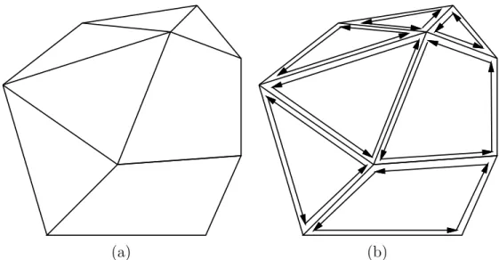
Figure 3.3: (a) A polyhedron can be described in terms of faces, edges, and vertices.
(b) The edges of each face can be stored in a circular list that is traversed in counterclockwise order with respect to the outward normal vector of the face.
Several data structures have been proposed that allow one to conveniently
“walk” around the polyhedral features. For example, the doubly connected edge list [264] data structure contains three types of records: faces, half-edges, and vertices. Intuitively, a half-edge is a directed edge. Each vertex record holds the point coordinates and a pointer to an arbitrary half-edge that touches the vertex.
Each face record contains a pointer to an arbitrary half-edge on its boundary. Each face is bounded by a circular list of half-edges. There is a pair of directed half-edge records for each edge of the polyhedon. Each half-edge is shown as an arrow in Figure 3.3b. Each half-edge record contains pointers to five other records: 1) the vertex from which the half-edge originates; 2) the “twin” half-edge, which bounds the neighboring face, and has the opposite direction; 3) the face that is bounded by the half-edge; 4) the next element in the circular list of edges that bound the face;
and 5) the previous element in the circular list of edges that bound the face. Once all of these records have been defined, one can conveniently traverse the structure of the polyhedron.
Now consider a solid representation of a polyhedron. Suppose thatO is a con- vex polyhedron, as shown in Figure 3.3. A solid representation can be constructed from the vertices. Each face of O has at least three vertices along its boundary.
Assuming these vertices are not collinear, an equation of the plane that passes through them can be determined of the form
ax+by+cz+d= 0, (3.7)
in whicha, b, c, d∈R are constants.
Once again,f can be constructed, except nowf :R3 →Rand
f(x, y, z) = ax+by+cz+d. (3.8)
3.1. GEOMETRIC MODELING 87 Letm be the number of faces. For each face of O, ahalf-space Hi is defined as a subset ofW:
Hi ={(x, y, z)∈ W |fi(x, y, z)≤0}. (3.9) It is important to choose fi so that it takes on negative values inside of the poly- hedron. In the case of a polygonal model, it was possible to consistently define fi by proceeding in counterclockwise order around the boundary. In the case of a polyhedron, the half-edge data structure can be used to obtain for each face the list of edges that form its boundary in counterclockwise order. Figure 3.3b shows the edge ordering for each face. For every edge, the arrows point in opposite directions, as required by the half-edge data structure. The equation for each face can be consistently determined as follows. Choose three consecutive vertices, p1, p2, p3 (they must not be collinear) in counterclockwise order on the boundary of the face. Let v12 denote the vector from p1 to p2, and let v23 denote the vector fromp2 to p3. The cross product v =v12×v23 always yields a vector that points out of the polyhedron and is normal to the face. Recall that the vector [a b c]
is parallel to the normal to the plane. If its components are chosen as a = v[1], b = v[2], and c = v[3], then f(x, y, z) ≤ 0 for all points in the half-space that contains the polyhedron.
As in the case of a polygonal model, a convex polyhedron can be defined as the intersection of a finite number of half-spaces, one for each face. A nonconvex polyhedron can be defined as the union of a finite number of convex polyhedra.
The predicate φ(x, y, z) can be defined in a similar manner, in this case yielding true if (x, y, z)∈ O, and false otherwise.
3.1.2 Semi-Algebraic Models
In both the polygonal and polyhedral models, f was a linear function. In the case of a semi-algebraic model for a 2D world,f can be any polynomial with real- valued coefficients and variables xand y. For a 3D world, f is a polynomial with variablesx, y, and z. The class of semi-algebraic models includes both polygonal and polyhedral models, which use first-degree polynomials. A point set determined by a single polynomial primitive is called analgebraic set; a point set that can be obtained by a finite number of unions and intersections of algebraic sets is called asemi-algebraic set.
Consider the case of a 2D world. A solid representation can be defined using algebraic primitivesof the form
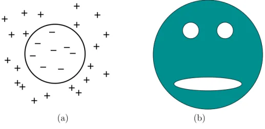
H ={(x, y)∈ W |f(x, y)≤0}. (3.10) As an example, let f = x2 +y2−4. In this case, H represents a disc of radius 2 that is centered at the origin. This corresponds to the set of points (x, y) for which f(x, y)≤0, as depicted in Figure 3.4a.
Example 3.1 (Gingerbread Face) Consider constructing a model of the shaded region shown in Figure 3.4b. Let the center of the outer circle have radius r1 and
+
+ + +
+ + + +
−
−
− −
−
−
− + −
+
+ + +
+ +
+ + +
+ + +
(a) (b)
Figure 3.4: (a) Once again,f is used to partitionR2 into two regions. In this case, the algebraic primitive represents a disc-shaped region. (b) The shaded “face” can be exactly modeled using only four algebraic primitives.
be centered at the origin. Suppose that the “eyes” have radius r2 and r3 and are centered at (x2, y2) and (x3, y3), respectively. Let the “mouth” be an ellipse with major axisa and minor axisb and is centered at (0, y4). The functions are defined as
f1 =x2+y2−r12,
f2 =− (x−x2)2+ (y−y2)2−r22 , f3 =− (x−x3)2+ (y−y3)2−r32
, f4 =− x2/a2+ (y−y4)2/b2−1
.
(3.11)
Forf2,f3, andf4, the familiar circle and ellipse equations were multiplied by−1 to yield algebraic primitives for all points outside of the circle or ellipse. The shaded regionO is represented as
O =H1∩H2∩H3∩H4. (3.12) In the case of semi-algebraic models, the intersection of primitives does not necessarily result in a convex subset of W. In general, however, it might be necessary to formO by taking unions and intersections of algebraic primitives.
A logical predicate, φ(x, y), can once again be formed, and collision checking is still performed in time that is linear in the number of primitives. Note that it is still very efficient to evaluate every primitive; f is just a polynomial that is evaluated on the point (x, y, z).
The semi-algebraic formulation generalizes easily to the case of a 3D world.
This results in algebraic primitives of the form
H ={(x, y, z)∈ W |f(x, y, z)≤0}, (3.13)
3.1. GEOMETRIC MODELING 89 which can be used to define a solid representation of a 3D obstacleO and a logical predicate φ.
Equations (3.10) and (3.13) are sufficient to express any model of interest. One may define many other primitives based on different relations, such asf(x, y, z)≥ 0, f(x, y, z) = 0, f(x, y, z) < 0, f(x, y, z) = 0, and f(x, y, z) 6= 0; however, most of them do not enhance the set of models that can be expressed. They might, however, be more convenient in certain contexts. To see that some primitives do not allow new models to be expressed, consider the primitive
H ={(x, y, z)∈ W |f(x, y, z)≥0}. (3.14) The right part may be alternatively represented as −f(x, y, z)≤ 0, and −f may be considered as a new polynomial function ofx, y, and z. For an example that involves the = relation, consider the primitive
H ={(x, y, z)∈ W |f(x, y, z) = 0}. (3.15) It can instead be constructed as H=H1∩H2, in which
H1 ={(x, y, z)∈ W |f(x, y, z)≤0} (3.16) and
H2 ={(x, y, z)∈ W | −f(x, y, z)≤0}. (3.17) The relation<does add some expressive power if it is used to construct primitives.2 It is needed to construct models that do not include the outer boundary (for example, the set of all pointsinside of a sphere, which does not include pointson the sphere). These are generally called open sets and are defined Chapter 4.
3.1.3 Other Models
The choice of a model often depends on the types of operations that will be per- formed by the planning algorithm. For combinatorial motion planning methods, to be covered in Chapter 6, the particular representation is critical. On the other hand, for sampling-based planning methods, to be covered in Chapter 5, the par- ticular representation is important only to the collision detection algorithm, which is treated as a “black box” as far as planning is concerned. Therefore, the models given in the remainder of this section are more likely to appear in sampling-based approaches and may be invisible to the designer of a planning algorithm (although it is never wise to forget completely about the representation).
2An alternative that yields the same expressive power is to still use ≤, but allow set comple- ments, in addition to unions and intersections.
Figure 3.5: A polygon with holes can be expressed by using different orientations:
counterclockwise for the outer boundary and clockwise for the hole boundaries.
Note that the shaded part is always to the left when following the arrows.
Nonconvex polygons and polyhedra The method in Section 3.1.1 required nonconvex polygons to be represented as a union of convex polygons. Instead, a boundary representation of a nonconvex polygon may be directly encoded by list- ing vertices in a specific order; assume that counterclockwise order is used. Each polygon of m vertices may be encoded by a list of the form (x1, y1), (x2, y2), . . ., (xm, ym). It is assumed that there is an edge between each (xi, yi) and (xi+1, yi+1) for eachifrom 1 tom−1, and also an edge between (xm, ym) and (x1, y1). Ordinar- ily, the vertices should be chosen in a way that makes the polygonsimple, meaning that no edges intersect. In this case, there is a well-defined interior of the polygon, which is to the left of every edge, if the vertices are listed in counterclockwise order.
What if a polygon has a hole in it? In this case, the boundary of the hole can be expressed as a polygon, but with its vertices appearing in the clockwise direction. To the left of each edge is the interior of the outer polygon, and to the right is the hole, as shown in Figure 3.5
Although the data structures are a little more complicated for three dimen- sions, boundary representations of nonconvex polyhedra may be expressed in a similar manner. In this case, instead of an edge list, one must specify faces, edges, and vertices, with pointers that indicate their incidence relations. Consistent ori- entations must also be chosen, and holes may be modeled once again by selecting opposite orientations.
3D triangles Suppose W =R3. One of the most convenient geometric models to express is a set of triangles, each of which is specified by three points, (x1, y1, z1), (x2, y2, z2), (x3, y3, z3). This model has been popular in computer graphics because graphics acceleration hardware primarily uses triangle primitives. It is assumed that the interior of the triangle is part of the model. Thus, two triangles are considered as “colliding” if one pokes into the interior of another. This model offers great flexibility because there are no constraints on the way in which triangles must
3.1. GEOMETRIC MODELING 91
Figure 3.6: Triangle strips and triangle fans can reduce the number of redundant points.
be expressed; however, this is also one of the drawbacks. There is no coherency that can be exploited to easily declare whether a point is “inside” or “outside” of a 3D obstacle. If there is at least some coherency, then it is sometimes preferable to reduce redundancy in the specification of triangle coordinates (many triangles will share the same corners). Representations that remove this redundancy are called a triangle strip, which is a sequence of triangles such that each adjacent pair shares a common edge, and a triangle fan, which is a triangle strip in which all triangles share a common vertex. See Figure 3.6.
Nonuniform rational B-splines (NURBS) These are used in many engi- neering design systems to allow convenient design and adjustment of curved sur- faces, in applications such as aircraft or automobile body design. In contrast to semi-algebraic models, which are implicit equations, NURBS and other splines are parametric equations. This makes computations such as rendering easier; however, others, such as collision detection, become more difficult. These models may be defined in any dimension. A brief 2D formulation is given here.
A curve can be expressed as
C(u) = Xn
i=0
wiPiNi,k(u) Xn
i=0
wiNi,k(u)
, (3.18)
in which wi ∈ R are weights and Pi are control points. The Ni,k are normalized basis functions of degreek, which can be expressed recursively as
Ni,k(u) =
u−ti
ti+k−ti
Ni,k−1(u) +
ti+k+1−u
ti+k+1−ti+1
Ni+1,k−1(u). (3.19)
The basis of the recursion isNi,0(u) = 1 ifti ≤u < ti+1, andNi,0(u) = 0 otherwise.
A knot vector is a nondecreasing sequence of real values, {t0, t1, . . . , tm}, that controls the intervals over which certain basic functions take effect.
Bitmaps For either W =R2 or W = R3, it is possible to discretize a bounded portion of the world into rectangular cells that may or may not be occupied.
The resulting model looks very similar to Example 2.1. The resolution of this discretization determines the number of cells per axis and the quality of the ap- proximation. The representation may be considered as a binary image in which
each “1” in the image corresponds to a rectangular region that contains at least one point ofO, and “0” represents those that do not contain any of O. Although bitmaps do not have the elegance of the other models, they often arise in applica- tions. One example is a digital map constructed by a mobile robot that explores an environment with its sensors. One generalization of bitmaps is a gray-scale map or occupancy grid. In this case, a numerical value may be assigned to each cell, indicating quantities such as “the probability that an obstacle exists” or the
“expected difficulty of traversing the cell.” The latter interpretation is often used in terrain maps for navigating planetary rovers.
Superquadrics Instead of using polynomials to define fi, many generalizations can be constructed. One popular primitive is a superquadric, which generalizes quadric surfaces. One example is a superellipsoid, which is given for W =R3 by
|x/a|n1 +|y/b|n2n1/n2
+|z/c|n1 −1≤0, (3.20) in whichn1 ≥2 and n2 ≥2. If n1 =n2 = 2, an ellipse is generated. As n1 and n2
increase, the superellipsoid becomes shaped like a box with rounded corners.
Generalized cylinders Ageneralized cylinderis a generalization of an ordinary cylinder. Instead of being limited to a line, the center axis is a continuous spine curve, (x(s), y(s), z(s)), for some parameters∈[0,1]. Instead of a constant radius, a radius function r(s) is defined along the spine. The value r(s) is the radius of the circle obtained as the cross section of the generalized cylinder at the point (x(s), y(s), z(s)). The normal to the cross-section plane is the tangent to the spine curve at s.
3.2 Rigid-Body Transformations
Any of the techniques from Section 3.1 can be used to define both the obstacle region and the robot. LetO refer to the obstacle region, which is a subset of W. Let A refer to the robot, which is a subset of R2 or R3, matching the dimension ofW. Although O remains fixed in the world, W, motion planning problems will require “moving” the robot,A.
3.2.1 General Concepts
Before giving specific transformations, it will be helpful to define them in general to avoid confusion in later parts when intuitive notions might fall apart. Suppose that a rigid robot,A, is defined as a subset of R2 orR3. Arigid-body transformation is a function,h:A → W, that maps every point ofAintoW with two requirements:
1) The distance between any pair of points of A must be preserved, and 2) the orientation of A must be preserved (no “mirror images”).
3.2. RIGID-BODY TRANSFORMATIONS 93 Using standard function notation, h(a) for some a ∈ A refers to the point in W that is “occupied” by a. Let
h(A) = {h(a)∈ W |a∈ A}, (3.21) which is the image ofhand indicates all points in W occupied by the transformed robot.
Transforming the robot model Consider transforming a robot model. If A is expressed by naming specific points inR2, as in a boundary representation of a polygon, then each point is simply transformed from a toh(a)∈ W. In this case, it is straightforward to transform the entire model using h. However, there is a slight complication if the robot model is expressed using primitives, such as
Hi ={a∈R2 |fi(a)≤0}. (3.22) This differs slightly from (3.2) because the robot is defined in R2 (which is not necessarilyW), and also a is used to denote a point (x, y)∈ A. Under a transfor- mationh, the primitive is transformed as
h(Hi) = {h(a)∈ W |fi(a)≤0}. (3.23) To transform the primitive completely, however, it is better to directly name points inw∈ W, as opposed toh(a)∈ W. Using the fact thata =h−1(w), this becomes h(Hi) ={w∈ W |fi(h−1(w))≤0}, (3.24) in which the inverse ofhappears in the right side because the original point a∈A needs to be recovered to evaluate fi. Therefore, it is important to be careful because either h or h−1 may be required to transform the model. This will be observed in more specific contexts in some coming examples.
A parameterized family of transformations It will become important to study families of transformations, in which some parameters are used to select the particular transformation. Therefore, it makes sense to generalizeh to accept two variables: a parameter vector, q ∈ Rn, along with a ∈ A. The resulting transformed point a is denoted by h(q, a), and the entire robot is transformed to h(q,A)⊂ W.
The coming material will use the following shorthand notation, which requires the specifichto be inferred from the context. Leth(q, a) be shortened toa(q), and leth(q,A) be shortened toA(q). This notation makes it appear that by adjusting the parameterq, the robotA travels around inW as different transformations are selected from the predetermined family. This is slightly abusive notation, but it is convenient. The expression A(q) can be considered as a set-valued function that yields the set of points in W that are occupied by A when it is transformed by q. Most of the time the notation does not cause trouble, but when it does, it is helpful to remember the definitions from this section, especially when trying to determine whether h orh−1 is needed.
Defining frames It was assumed so far thatAis defined inR2 orR3, but before it is transformed, it is not considered to be a subset of W. The transformation h places the robot in W. In the coming material, it will be convenient to indicate this distinction using coordinate frames. The origin and coordinate basis vectors ofW will be referred to as the world frame.3 Thus, any pointw∈ W is expressed in terms of the world frame.
The coordinates used to define A are initially expressed in the body frame, which represents the origin and coordinate basis vectors of R2 or R3. In the case of A ⊂ R2, it can be imagined that the body frame is painted on the robot.
Transforming the robot is equivalent to converting its model from the body frame to the world frame. This has the effect of placing4 A into W at some position and orientation. When multiple bodies are covered in Section 3.3, each body will have its own body frame, and transformations require expressing all bodies with respect to the world frame.
3.2.2 2D Transformations
Translation A rigid robotA ⊂R2istranslatedby using two parameters,xt, yt∈ R. Using definitions from Section 3.2.1,q = (xt, yt), and h is defined as
h(x, y) = (x+xt, y+yt). (3.25) A boundary representation ofA can be translated by transforming each vertex in the sequence of polygon vertices using (3.25). Each point, (xi, yi), in the sequence is replaced by (xi+xt, yi+yt).
Now consider a solid representation ofA, defined in terms of primitives. Each primitive of the form
Hi ={(x, y)∈R2 |f(x, y)≤0} (3.26) is transformed to
h(Hi) = {(x, y)∈ W |f(x−xt, y−yt)≤0}. (3.27) Example 3.2 (Translating a Disc) For example, suppose the robot is a disc of unit radius, centered at the origin. It is modeled by a single primitive,
Hi ={(x, y)∈R2 |x2 +y2−1≤0}. (3.28) Suppose A = Hi is translated xt units in the x direction and yt units in the y direction. The transformed primitive is
h(Hi) ={(x, y)∈ W |(x−xt)2+ (y−yt)2−1≤0}, (3.29)
3The world frame serves the same purpose as an inertial frame in Newtonian mechanics.
Intuitively, it is a frame that remains fixed and from which all measurements are taken. See Section 13.3.1.
4Technically, this placement is a function called an orientation-preserving isometric embed- ding.
3.2. RIGID-BODY TRANSFORMATIONS 95
Moving the Robot
Moving the Coordinate Frame
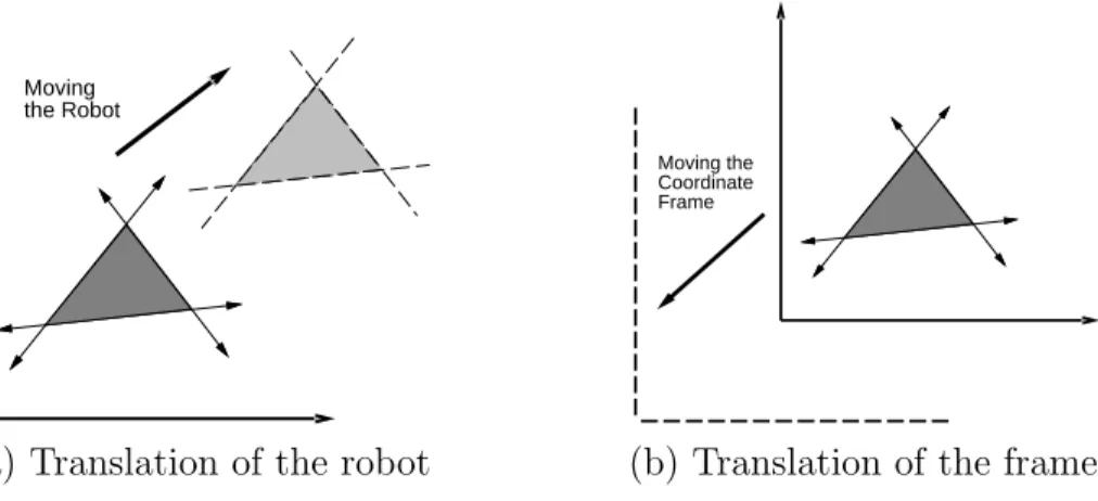
(a) Translation of the robot (b) Translation of the frame
Figure 3.7: Every transformation has two interpretations.
which is the familiar equation for a disc centered at (xt, yt). In this example, the inverse, h−1 is used, as described in Section 3.2.1.
The translated robot is denoted asA(xt, yt). Translation by (0,0) is the iden- tity transformation, which results in A(0,0) = A, if it is assumed that A ⊂ W (recall thatA does not necessarily have to be initially embedded inW). It will be convenient to use the termdegrees of freedomto refer to the maximum number of independent parameters that are needed to completely characterize the transfor- mation applied to the robot. If the set of allowable values for xt and yt forms a two-dimensional subset ofR2, then the degrees of freedom is two.
Suppose that A is defined directly in W with translation. As shown in Figure 3.7, there are two interpretations of a rigid-body transformation applied toA: 1) The world frame remains fixed and the robot is transformed; 2) the robot remains fixed and the world frame is translated. The first one characterizes the effect of the transformation from a fixed world frame, and the second one indicates how the transformation appears from the robot’s perspective. Unless stated otherwise, the first interpretation will be used when we refer to motion planning problems because it often models a robot moving in a physical world. Numerous books cover coordinate transformations under the second interpretation. This has been known to cause confusion because the transformations may sometimes appear “backward”
from what is desired in motion planning.
Rotation The robot, A, can be rotated counterclockwise by some angle θ ∈ [0,2π) by mapping every (x, y)∈ A as
(x, y)7→(xcosθ−ysinθ, xsinθ+ycosθ). (3.30)
Using a 2×2 rotation matrix, R(θ) =
cosθ −sinθ sinθ cosθ
, (3.31)
the transformation can be written as xcosθ−ysinθ
xsinθ+ycosθ
=R(θ) x
y
. (3.32)
Using the notation of Section 3.2.1, R(θ) becomes h(q), for which q = θ. For linear transformations, such as the one defined by (3.32), recall that the column vectors represent the basis vectors of the new coordinate frame. The column vectors ofR(θ) are unit vectors, and their inner product (or dot product) is zero, indicating that they are orthogonal. Suppose that the x and y coordinate axes, which represent the body frame, are “painted” onA. The columns ofR(θ) can be derived by considering the resulting directions of the x- and y-axes, respectively, after performing a counterclockwise rotation by the angle θ. This interpretation generalizes nicely for higher dimensional rotation matrices.
Note that the rotation is performed about the origin. Thus, when defining the model of A, the origin should be placed at the intended axis of rotation. Using the semi-algebraic model, the entire robot model can be rotated by transforming each primitive, yielding A(θ). The inverse rotation, R(−θ), must be applied to each primitive.
Combining translation and rotation Suppose a rotation by θ is performed, followed by a translation by xt, yt. This can be used to place the robot in any desired position and orientation. Note that translations and rotations do not commute! If the operations are applied successively, each (x, y)∈ Ais transformed
to
xcosθ−ysinθ+xt
xsinθ+ycosθ+yt
. (3.33)
The following matrix multiplication yields the same result for the first two vector components:
cosθ −sinθ xt
sinθ cosθ yt
0 0 1
x y 1
=
xcosθ−ysinθ+xt
xsinθ+ycosθ+yt
1
. (3.34) This implies that the 3×3 matrix,
T =
cosθ −sinθ xt
sinθ cosθ yt
0 0 1
, (3.35)
represents a rotation followed by a translation. The matrix T will be referred to as a homogeneous transformation matrix. It is important to remember that T
3.2. RIGID-BODY TRANSFORMATIONS 97
Yaw z
y
x
Pitch Roll
γ
β α
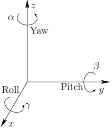
Figure 3.8: Any three-dimensional rotation can be described as a sequence of yaw, pitch, and roll rotations.
represents a rotationfollowed by a translation (not the other way around). Each primitive can be transformed using the inverse of T, resulting in a transformed solid model of the robot. The transformed robot is denoted by A(xt, yt, θ), and in this case there are three degrees of freedom. The homogeneous transformation matrix is a convenient representation of the combined transformations; therefore, it is frequently used in robotics, mechanics, computer graphics, and elsewhere.
It is called homogeneous because over R3 it is just a linear transformation with- out any translation. The trick of increasing the dimension by one to absorb the translational part is common in projective geometry [804].
3.2.3 3D Transformations
Rigid-body transformations for the 3D case are conceptually similar to the 2D case;
however, the 3D case appears more difficult because rotations are significantly more complicated.
3D translation The robot, A, is translatedby some xt, yt, zt∈R using
(x, y, z)7→(x+xt, y+yt, z+zt). (3.36) A primitive of the form
Hi ={(x, y, z)∈ W |fi(x, y, z)≤0} (3.37) is transformed to
{(x, y, z)∈ W |fi(x−xt, y−yt, z−zt)≤0}. (3.38) The translated robot is denoted as A(xt, yt, zt).
Yaw, pitch, and roll rotations A 3D body can be rotated about three orthog- onal axes, as shown in Figure 3.8. Borrowing aviation terminology, these rotations will be referred to as yaw, pitch, and roll:
1. A yaw is a counterclockwise rotation of α about the z-axis. The rotation matrix is given by
Rz(α) =
cosα −sinα 0 sinα cosα 0
0 0 1
. (3.39)
Note that the upper left entries of Rz(α) form a 2D rotation applied to the x and y coordinates, whereas thez coordinate remains constant.
2. A pitch is a counterclockwise rotation of β about the y-axis. The rotation matrix is given by
Ry(β) =
cosβ 0 sinβ
0 1 0
−sinβ 0 cosβ
. (3.40)
3. A roll is a counterclockwise rotation of γ about the x-axis. The rotation matrix is given by
Rx(γ) =
1 0 0
0 cosγ −sinγ 0 sinγ cosγ
. (3.41)
Each rotation matrix is a simple extension of the 2D rotation matrix, (3.31). For example, the yaw matrix, Rz(α), essentially performs a 2D rotation with respect to the x and y coordinates while leaving the z coordinate unchanged. Thus, the third row and third column of Rz(α) look like part of the identity matrix, while the upper right portion ofRz(α) looks like the 2D rotation matrix.
The yaw, pitch, and roll rotations can be used to place a 3D body in any orientation. A single rotation matrix can be formed by multiplying the yaw, pitch, and roll rotation matrices to obtain
R(α,β, γ) = Rz(α)Ry(β)Rx(γ) =
cosαcosβ cosαsinβsinγ−sinαcosγ cosαsinβcosγ+ sinαsinγ sinαcosβ sinαsinβsinγ+ cosαcosγ sinαsinβcosγ−cosαsinγ
−sinβ cosβsinγ cosβcosγ
.
(3.42) It is important to note thatR(α, β, γ) performs the roll first, then the pitch, and finally the yaw. If the order of these operations is changed, a different rotation
3.2. RIGID-BODY TRANSFORMATIONS 99 matrix would result. Be careful when interpreting the rotations. Consider the final rotation, a yaw by α. Imagine sitting inside of a robot A that looks like an aircraft. If β = γ = 0, then the yaw turns the plane in a way that feels like turning a car to the left. However, for arbitrary values of β and γ, the final rotation axis will not be vertically aligned with the aircraft because the aircraft is left in an unusual orientation beforeα is applied. The yaw rotation occurs about thez-axis of the world frame, not the body frame of A. Each time a new rotation matrix is introduced from the left, it has no concern for original body frame of A. It simply rotates every point inR3 in terms of the world frame. Note that 3D rotations depend on three parameters,α, β, and γ, whereas 2D rotations depend only on a single parameter, θ. The primitives of the model can be transformed using R(α, β, γ), resulting in A(α, β, γ).
Determining yaw, pitch, and roll from a rotation matrix It is often con- venient to determine the α, β, and γ parameters directly from a given rotation matrix. Suppose an arbitrary rotation matrix
r11 r12 r13
r21 r22 r23
r31 r32 r33
(3.43)
is given. By setting each entry equal to its corresponding entry in (3.42), equations are obtained that must be solved for α, β, and γ. Note that r21/r11 = tanα and r32/r33 = tanγ. Also, r31 = −sinβ and p
r322 +r332 = cosβ. Solving for each angle yields
α= tan−1(r21/r11), (3.44) β = tan−1
−r31
q
r232+r233
, (3.45)
and
γ = tan−1(r32/r33). (3.46) There is a choice of four quadrants for the inverse tangent functions. How can the correct quadrant be determined? Each quadrant should be chosen by using the signs of the numerator and denominator of the argument. The numerator sign selects whether the direction will be above or below the x-axis, and the denomi- nator selects whether the direction will be to the left or right of the y-axis. This is the same as the atan2 function in the C programming language, which nicely expands the range of the arctangent to [0,2π). This can be applied to express (3.44), (3.45), and (3.46) as
α= atan2(r21, r11), (3.47)
β = atan2
−r31, q
r232+r233
, (3.48)
and
γ = atan2(r32, r33). (3.49)
Note that this method assumes r116= 0 and r33 6= 0.
The homogeneous transformation matrix for 3D bodies As in the 2D case, a homogeneous transformation matrix can be defined. For the 3D case, a 4×4 matrix is obtained that performs the rotation given by R(α, β, γ), followed by a translation given by xt, yt, zt. The result is
T =
cosαcosβ cosαsinβsinγ−sinαcosγ cosαsinβcosγ+ sinαsinγ xt sinαcosβ sinαsinβsinγ+ cosαcosγ sinαsinβcosγ−cosαsinγ yt
−sinβ cosβsinγ cosβcosγ zt
0 0 0 1
.
(3.50) Once again, the order of operations is critical. The matrix T in (3.50) represents the following sequence of transformations:
1. Roll by γ 3. Yaw byα
2. Pitch byβ 4. Translate by (xt, yt, zt).
The robot primitives can be transformed to yieldA(xt, yt, zt, α, β, γ). A 3D rigid body that is capable of translation and rotation therefore has six degrees of free- dom.
3.3 Transforming Kinematic Chains of Bodies
The transformations become more complicated for a chain of attached rigid bodies.
For convenience, each rigid body is referred to as alink. LetA1,A2, . . . ,Amdenote a set ofmlinks. For eachisuch that 1≤i < m, linkAi is “attached” to linkAi+1 in a way that allowsAi+1 some constrained motion with respect toAi. The motion constraint must be explicitly given, and will be discussed shortly. As an example, imagine a trailer that is attached to the back of a car by a hitch that allows the trailer to rotate with respect to the car. In general, a set of attached bodies will be referred to as a linkage. This section considers bodies that are attached in a single chain. This leads to a particular linkage called akinematic chain.
3.3.1 A 2D Kinematic Chain
Before considering a kinematic chain, suppose A1 and A2 are unattached rigid bodies, each of which is capable of translating and rotating in W = R2. Since each body has three degrees of freedom, there is a combined total of six degrees of freedom; the independent parameters arex1, y1,θ1,x2, y2, and θ2.
Attaching bodies When bodies are attached in a kinematic chain, degrees of freedom are removed. Figure 3.9 shows two different ways in which a pair of 2D links can be attached. The place at which the links are attached is called a joint.
For arevolute joint, one link is capable only of rotation with respect to the other.
For a prismatic joint is shown, one link slides along the other. Each type of joint removes two degrees of freedom from the pair of bodies. For example, consider a
3.3. TRANSFORMING KINEMATIC CHAINS OF BODIES 101
A1
A2
A1
A2
Revolute Prismatic
Figure 3.9: Two types of 2D joints: a revolute joint allows one link to rotate with respect to the other, and a prismatic joint allows one link to translate with respect to the other.
revolute joint that connects A1 to A2. Assume that the point (0,0) in the body frame of A2 is permanently fixed to a point (xa, ya) in the body frame of A1. This implies that the translation of A2 is completely determined once xa and ya
are given. Note that xa and ya depend on x1, y1, and θ1. This implies that A1
and A2 have a total of four degrees of freedom when attached. The independent parameters are x1, y1, θ1, and θ2. The task in the remainder of this section is to determine exactly how the models ofA1, A2, . . .,Am are transformed when they are attached in a chain, and to give the expressions in terms of the independent parameters.
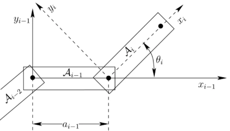
Consider the case of a kinematic chain in which each pair of links is attached by a revolute joint. The first task is to specify the geometric model for each link, Ai. Recall that for a single rigid body, the origin of the body frame determines the axis of rotation. When defining the model for a link in a kinematic chain, excessive complications can be avoided by carefully placing the body frame. Since rotation occurs about a revolute joint, a natural choice for the origin is the joint between Ai and Ai−1 for each i > 1. For convenience that will soon become evident, the xi-axis for the body frame ofAi is defined as the line through the two joints that lie in Ai, as shown in Figure 3.10. For the last link, Am, the xm-axis can be placed arbitrarily, assuming that the origin is placed at the joint that connects Am to Am−1. The body frame for the first link, A1, can be placed using the same considerations as for a single rigid body.
Homogeneous transformation matrices for 2D chains We are now pre- pared to determine the location of each link. The location in W of a point in (x, y)∈ A1 is determined by applying the 2D homogeneous transformation matrix (3.35),
T1 =
cosθ1 −sinθ1 xt
sinθ1 cosθ1 yt
0 0 1
. (3.51)
xi−1 θi
Ai−1 Ai−2
xi yi
ai−1 yi−1
Ai
Figure 3.10: The body frame of eachAi, for 1< i < m, is based on the joints that connectAi to Ai−1 and Ai+1.
As shown in Figure 3.10, letai−1 be the distance between the joints in Ai−1. The orientation difference between Ai and Ai−1 is denoted by the angle θi. Let Ti
represent a 3×3 homogeneous transformation matrix (3.35), specialized for link Ai for 1< i≤m,
Ti =
cosθi −sinθi ai−1
sinθi cosθi 0
0 0 1
. (3.52)
This generates the following sequence of transformations:
1. Rotate counterclockwise by θi. 2. Translate by ai−1 along the x-axis.
The transformationTi expresses the difference between the body frame ofAi and the body frame of Ai−1. The application of Ti moves Ai from its body frame to the body frame ofAi−1. The application ofTi−1Ti moves bothAi and Ai−1 to the body frame of Ai−2. By following this procedure, the location in W of any point (x, y)∈ Am is determined by multiplying the transformation matrices to obtain
T1T2· · ·Tm
x y 1
. (3.53)
Example 3.3 (A 2D Chain of Three Links) To gain an intuitive understand- ing of these transformations, consider determining the configuration for link A3, as shown in Figure 3.11. Figure 3.11a shows a three-link chain in which A1 is at its initial configuration and the other links are each offset by π/4 from the pre- vious link. Figure 3.11b shows the frame in which the model for A3 is initially defined. The application of T3 causes a rotation of θ3 and a translation by a2. As shown in Figure 3.11c, this places A3 in its appropriate configuration. Note that A2 can be placed in its initial configuration, and it will be attached cor- rectly to A3. The application of T2 to the previous result places both A3 and A2
3.3. TRANSFORMING KINEMATIC CHAINS OF BODIES 103 in their proper configurations, andA1 can be placed in its initial configuration.
For revolute joints, theai parameters are constants, and theθi parameters are variables. The transformed mth link is represented as Am(xt, yt, θ1, . . . , θm). In some cases, the first link might have a fixed location in the world. In this case, the revolute joints account for all degrees of freedom, yieldingAm(θ1, . . . , θm). For prismatic joints, the ai parameters are variables, instead of the θi parameters. It is straightforward to include both types of joints in the same kinematic chain.
3.3.2 A 3D Kinematic Chain
As for a single rigid body, the 3D case is significantly more complicated than the 2D case due to 3D rotations. Also, several more types of joints are possible, as shown in Figure 3.12. Nevertheless, the main ideas from the transformations of 2D kinematic chains extend to the 3D case. The following steps from Section 3.3.1 will be recycled here:
1. The body frame must be carefully placed for each Ai.
2. Based on joint relationships, several parameters are measured.
3. The parameters define a homogeneous transformation matrix, Ti.
4. The location in W of any point in Am is given by applying the matrix T1T2· · ·Tm.
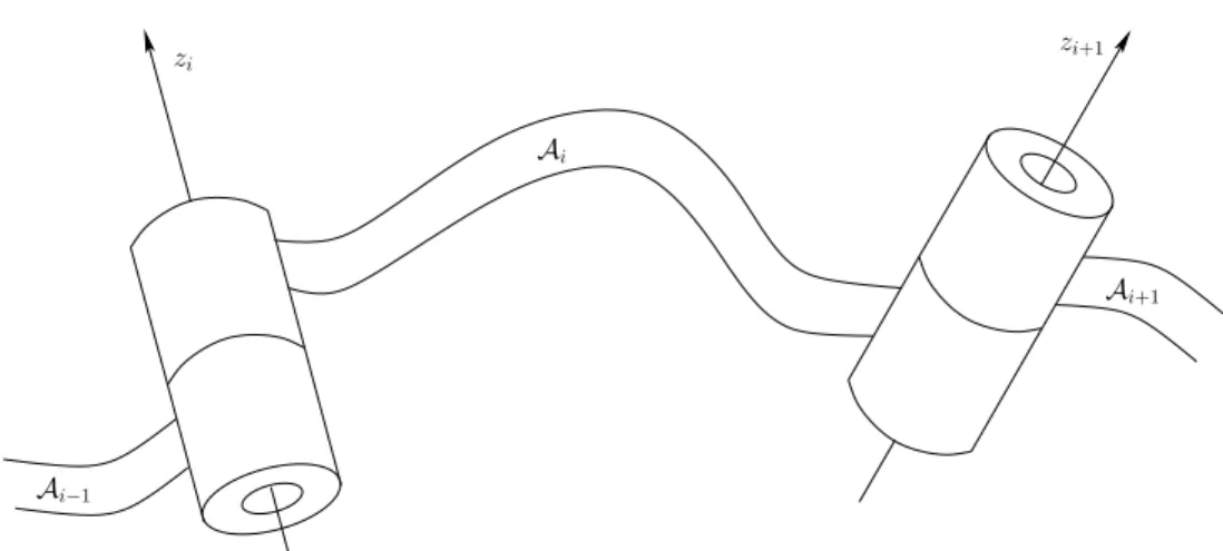
Consider a kinematic chain of m links in W = R3, in which each Ai for 1 ≤ i < m is attached to Ai+1 by a revolute joint. Each link can be a complicated, rigid body as shown in Figure 3.13. For the 2D problem, the coordinate frames were based on the points of attachment. For the 3D problem, it is convenient to use the axis of rotation of each revolute joint (this is equivalent to the point of attachment for the 2D case). The axes of rotation will generally be skew lines in R3, as shown in Figure 3.14. Let thezi-axis be the axis of rotation for the revolute joint that holdsAi toAi−1. Between each pair of axes in succession, let thexi-axis join the closest pair of points between thezi- andzi+1-axes, with the origin on the zi-axis and the direction pointing towards the nearest point of the zi+1-axis. This axis is uniquely defined if thezi- andzi+1-axes are not parallel. The recommended body frame for each Ai will be given with respect to the zi- and xi-axes, which are shown in Figure 3.14. Assuming a right-handed coordinate system, the yi- axis points away from us in Figure 3.14. In the transformations that will appear shortly, the coordinate frame given by xi, yi, and zi will be most convenient for defining the model for Ai. It might not always appear convenient because the origin of the frame may even lie outside of Ai, but the resulting transformation matrices will be easy to understand.
In Section 3.3.1, each Ti was defined in terms of two parameters, ai−1 and θi. For the 3D case, four parameters will be defined: di, θi, ai−1, and αi−1. These
x3
θ3
θ2
A1
A2 y1
x1
x2
A3
A3 y3
x3
(a) A three-link chain (b) A3 in its body frame
A2
A3 y2
x2
A1
A2 A3 y1
x1
(c) T3 puts A3 inA2’s body frame (d) T2T3 puts A3 in A1’s body frame Figure 3.11: Applying the transformation T2T3 to the model of A3. If T1 is the identity matrix, then this yields the location in W of points in A3.
3.3. TRANSFORMING KINEMATIC CHAINS OF BODIES 105
Revolute Prismatic Screw
1 Degree of Freedom 1 Degree of Freedom 1 Degree of Freedom
Cylindrical Spherical Planar
2 Degrees of Freedom 3 Degrees of Freedom 3 Degrees of Freedom Figure 3.12: Types of 3D joints arising from the 2D surface contact between two bodies.
are referred to as Denavit-Hartenberg (DH) parameters [434]. The definition of each parameter is indicated in Figure 3.15. Figure 3.15a shows the definition of di. Note that thexi−1- andxi-axes contact the zi-axis at two different places. Let di denote signed distance between these points of contact. If the xi-axis is above the xi−1-axis along the zi-axis, then di is positive; otherwise, di is negative. The parameterθi is the angle between thexi- andxi−1-axes, which corresponds to the rotation about the zi-axis that moves the xi−1-axis to coincide with the xi-axis.
The parameter ai is the distance between the zi- and zi−1-axes; recall these are generally skew lines in R3. The parameter αi−1 is the angle between the zi- and zi−1-axes.
Two screws The homogeneous transformation matrixTi will be constructed by combining two simpler transformations. The transformation
Ri =
cosθi −sinθi 0 0 sinθi cosθi 0 0
0 0 1 di
0 0 0 1
(3.54)
causes a rotation of θi about the zi-axis, and a translation of di along the zi- axis. Notice that the rotation byθi and translation by di commute because both
Ai+1 zi+1 zi
Ai−1
Ai
Figure 3.13: The rotation axes for a generic link attached by revolute joints.
operations occur with respect to the same axis, zi. The combined operation of a translation and rotation with respect to the same axis is referred to as ascrew (as in the motion of a screw through a nut). The effect of Ri can thus be considered as a screw about thezi-axis. The second transformation is
Qi−1 =
1 0 0 ai−1
0 cosαi−1 −sinαi−1 0 0 sinαi−1 cosαi−1 0
0 0 0 1
, (3.55)
which can be considered as a screw about the xi−1-axis. A rotation ofαi−1 about the xi−1-axis and a translation of ai−1 are performed.
The homogeneous transformation matrix The transformation Ti, for each isuch that 1 < i≤m, is
Ti =Qi−1Ri =
cosθi −sinθi 0 ai−1
sinθicosαi−1 cosθicosαi−1 −sinαi−1 −sinαi−1di
sinθisinαi−1 cosθisinαi−1 cosαi−1 cosαi−1di
0 0 0 1
. (3.56) This can be considered as the 3D counterpart to the 2D transformation matrix, (3.52). The following four operations are performed in succession:
1. Translate by di along the zi-axis.
2. Rotate counterclockwise by θi about thezi-axis.
3. Translate by ai−1 along the xi−1-axis.
4. Rotate counterclockwise by αi−1 about thexi−1-axis.
3.3. TRANSFORMING KINEMATIC CHAINS OF BODIES 107
zi+1
xi zi
xi−1 zi−1
Figure 3.14: The rotation axes of the generic links are skew lines inR3. As in the 2D case, the first matrix, T1, is special. To represent any position and orientation of A1, it could be defined as a general rigid-body homogeneous transformation matrix, (3.50). If the first body is only capable of rotation via a revolute joint, then a simple convention is usually followed. Let thea0, α0 param- eters of T1 be assigned as a0 =α0 = 0 (there is no z0-axis). This implies that Q0
from (3.55) is the identity matrix, which makesT1 =R1.
The transformation Ti for i >1 gives the relationship between the body frame ofAi and the body frame ofAi−1. The position of a point (x, y, z) onAm is given by
T1T2· · ·Tm
x y z 1
. (3.57)
For each revolute joint,θi is treated as the only variable inTi. Prismatic joints can be modeled by allowingai to vary. More complicated joints can be modeled as a sequence of degenerate joints. For example, a spherical joint can be considered as a sequence of three zero-length revolute joints; the joints perform a roll, a pitch, and a yaw. Another option for more complicated joints is to abandon the DH representation and directly develop the homogeneous transformation matrix.
This might be needed to preserve topological properties that become important in Chapter 4.
Example 3.4 (Puma 560) This example demonstrates the 3D chain kinematics on a classic robot manipulator, the PUMA 560, shown in Figure 3.16. The cur- rent parameterization here is based on [37, 555]. The procedure is to determine