Chapter 4 The Configuration Space

(1)

Chapter 4 The Configuration Space

Chapter 3 only covered how to model and transform a collection of bodies; however, for the purposes of planning it is important to define the state space. The state space for motion planning is a set of possible transformations that could be applied to the robot. This will be referred to as theconfiguration space, based on Lagrangian mechanics and the seminal work of Lozano-Pérez [656, 660, 657], who extensively utilized this notion in the context of planning (the idea was also used in early collision avoidance work by Udupa [947]). The motion planning literature was further unified around this concept by Latombe’s book [588]. Once the configuration space is clearly understood, many motion planning problems that appear different in terms of geometry and kinematics can be solved by the same planning algorithms. This level of abstraction is therefore very important.

This chapter provides important foundational material that will be very useful in Chapters 5 to 8 and other places where planning over continuous state spaces occurs. Many concepts introduced in this chapter come directly from mathematics, particularly from topology. Therefore, Section 4.1 gives a basic overview of topological concepts. Section 4.2 uses the concepts from Chapter 3 to define the configuration space. After reading this, you should be able to precisely characterize the configuration space of a robot and understand its structure. In Section 4.3, obstacles in the world are transformed into obstacles in the configuration space, but it is important to understand that this transformation may not be explicitly constructed. The implicit representation of the state space is a recurring theme throughout planning. Section 4.4 covers the important case of kinematic chains that have loops, which was mentioned in Section 3.4. This case is so difficult that even the space of transformations usually cannot be explicitly characterized (i.e., parameterized).

4.1 Basic Topological Concepts

This section introduces basic topological concepts that are helpful in understanding conﬁguration spaces. Topology is a challenging subject to understand in depth.

The treatment given here provides only a brief overview and is designed to stim- 127

(2)

ulate further study (see the literature overview at the end of the chapter). To advance further in this chapter, it is not necessary to understand all of the material of this section; however, the more you understand, the deeper will be your understanding of motion planning in general.

4.1.1 Topological Spaces

Recall the concepts of open and closed intervals in the set of real numbersR. The open interval (0,1) includes all real numbers between 0 and 1, except 0 and 1.

However, for either endpoint, an infinite sequence may be defined that converges to it. For example, the sequence 1/2, 1/4, . . ., 1/2ⁱ converges to 0 as i tends to infinity. This means that we can choose a point in (0,1) within any small, positive distance from 0 or 1, but we cannot pick one exactly on the boundary of the interval. For a closed interval, such as [0,1], the boundary points are included.

The notion of an open set lies at the heart of topology. The open set deﬁnition that will appear here is a substantial generalization of the concept of an open interval. The concept applies to a very general collection of subsets of some larger space. It is general enough to easily include any kind of conﬁguration space that may be encountered in planning.

A setX is called atopological spaceif there is a collection of subsets ofX called open sets for which the following axioms hold:

1. The union of any number of open sets is an open set.

2. The intersection of a ﬁnite number of open sets is an open set.

3. Both X and ∅ are open sets.

Note that in the first axiom, the union of an infinite number of open sets may be taken, and the result must remain an open set. Intersecting an infinite number of open sets, however, does not necessarily lead to an open set.

For the special case of X = R, the open sets include open intervals, as ex- pected. Many sets that are not intervals are open sets because taking unions and intersections of open intervals yields other open sets. For example, the set

[∞

i=1

1 3ⁱ, 2

3ⁱ

, (4.1)

which is an inﬁnite union of pairwise-disjoint intervals, is an open set.

Closed sets Open sets appear directly in the deﬁnition of a topological space.

It next seems that closed sets are needed. Suppose X is a topological space. A subsetC ⊂X is deﬁned to be aclosed setif and only ifX\C is an open set. Thus, the complement of any open set is closed, and the complement of any closed set is open. Any closed interval, such as [0,1], is a closed set because its complement, (−∞,0)∪ (1,∞), is an open set. For another example, (0,1) is an open set;

(3)

4.1. BASIC TOPOLOGICAL CONCEPTS 129

x₁

U

x3

x2

O2

O₁

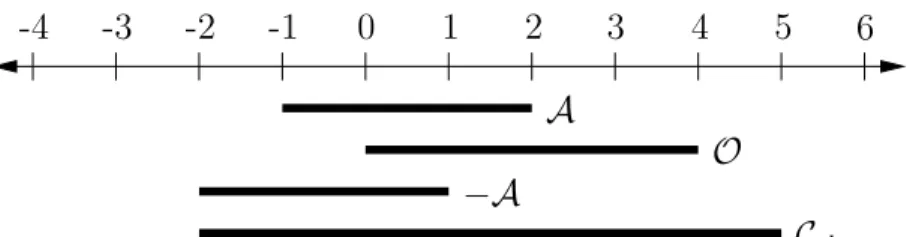
Figure 4.1: An illustration of the boundary deﬁnition. SupposeX =R², andU is a subset as shown. Three kinds of points appear: 1) x1 is a boundary point, 2) x2

is an interior point, and 3)x3 is an exterior point. Both x1 and x2 are limit points of U.

therefore, R\(0,1) = (−∞,0]∪[1,∞) is a closed set. The use of “(” may seem wrong in the last expression, but “[” cannot be used because −∞ and ∞ do not belong toR. Thus, the use of “(” is just a notational quirk.

Are all subsets of X either closed or open? Although it appears that open sets and closed sets are opposites in some sense, the answer is no. For X = R, the interval [0,2π) is neither open nor closed (consider its complement: [2π,∞) is closed, and (−∞,0) is open). Note that for any topological space, X and ∅ are both open and closed!

Special points From the deﬁnitions and examples so far, it should seem that points on the “edge” or “border” of a set are important. There are several terms that capture where points are relative to the border. LetX be a topological space, and letU be any subset ofX. Furthermore, letxbe any point inX. The following terms capture the position of point x relative to U (see Figure 4.1):

• If there exists an open set O1 such that x∈O1 andO1 ⊆U, thenx is called aninterior pointofU. The set of all interior points inU is called the interior of U and is denoted by int(U).

• If there exists an open set O2 such that x ∈ O2 and O2 ⊆ X\U, then x is called an exterior pointwith respect to U.

• If x is neither an interior point nor an exterior point, then it is called a boundary point of U. The set of all boundary points in X is called the boundary of U and is denoted by ∂U.

• All points in x ∈ X must be one of the three above; however, another term is often used, even though it is redundant given the other three. If xis either an interior point or a boundary point, then it is called a limit point(or accumulation point) ofU. The set of all limit points ofU is a closed set called the closureof U, and it is denoted by cl(U). Note that cl(U) = int(U)∪∂U. For the case ofX =R, the boundary points are the endpoints of intervals. For example, 0 and 1 are boundary points of intervals, (0,1), [0,1], [0,1), and (0,1].

Thus, U may or may not include its boundary points. All of the points in (0,1)

(4)

are interior points, and all of the points in [0,1] are limit points. The motivation of the name “limit point” comes from the fact that such a point might be the limit of an inﬁnite sequence of points in U. For example, 0 is the limit point of the sequence generated by 1/2ⁱ for each i∈N, the natural numbers.

There are several convenient consequences of the deﬁnitions. A closed set C contains the limit point of any sequence that is a subset of C. This implies that it contains all of its boundary points. The closure, cl, always results in a closed set because it adds all of the boundary points to the set. On the other hand, an open set contains none of its boundary points. These interpretations will come in handy when considering obstacles in the conﬁguration space for motion planning.

Some examples The deﬁnition of a topological space is so general that an incredible variety of topological spaces can be constructed.

Example 4.1 (The Topology of Rⁿ) We should expect that X = Rⁿ for any integer n is a topological space. This requires characterizing the open sets. An open ballB(x, ρ) is the set of points in the interior of a sphere of radiusρ, centered atx. Thus,

B(x, ρ) = {x^′ ∈Rⁿ| kx^′−xk< ρ}, (4.2) in which k · k denotes the Euclidean norm (or magnitude) of its argument. The open balls are open sets in Rⁿ. Furthermore, all other open sets can be expressed as a countable union of open balls.¹ For the case ofR, this reduces to representing any open set as a union of intervals, which was done so far.

Even though it is possible to express open sets ofRⁿas unions of balls, we pre- fer to use other representations, with the understanding that one could revert to open balls if necessary. The primitives of Section 3.1 can be used to generate many interesting open and closed sets. For example, any algebraic primitive expressed in the formH ={x∈Rⁿ | f(x)≤0} produces a closed set. Taking ﬁnite unions and intersections of these primitives will produce more closed sets. Therefore, all of the models from Sections 3.1.1 and 3.1.2 produce an obstacle region O that is a closed set. As mentioned in Section 3.1.2, sets constructed only from primitives

that use the< relation are open.

Example 4.2 (Subspace Topology) A new topological space can easily be constructed from a subset of a topological space. Let X be a topological space, and let Y ⊂ X be a subset. The subspace topology on Y is obtained by deﬁning the open sets to be every subset ofY that can be represented as U∩Y for some open set U ⊆ X. Thus, the open sets for Y are almost the same as for X, except that the points that do not lie in Y are trimmed away. New subspaces can be constructed by intersecting open sets of Rⁿ with a complicated region deﬁned by semi-algebraic models. This leads to many interesting topological spaces, some of

1Such a collection of balls is often referred to as a basis.

(5)

which will appear later in this chapter.

Example 4.3 (The Trivial Topology) For any setX, there is always one trivial example of a topological space that can be constructed from it. Declare that X and ∅are the only open sets. Note that all of the axioms are satisﬁed.

Example 4.4 (A Strange Topology) It is important to keep in mind the almost absurd level of generality that is allowed by the definition of a topological space. A topological space can be defined for any set, as long as the declared open sets obey the axioms. Suppose a four-element set is defined as

X ={cat,dog,tree,house}. (4.3) In addition to∅ and X, suppose that{cat} and {dog} are open sets. Using the axioms, {cat,dog} must also be an open set. Closed sets and boundary points can be derived for this topology once the open sets are deﬁned.

After the last example, it seems that topological spaces are so general that not much can be said about them. Most spaces that are considered in topology and analysis satisfy more axioms. For Rⁿ and any conﬁguration spaces that arise in this book, the following is satisﬁed:

Hausdorff axiom: For any distinct x₁, x₂ ∈X, there exist open sets O₁ and O2 such that x1 ∈O1, x2 ∈O2, and O1∩O2 =∅.

In other words, it is possible to separate x1 and x2 into nonoverlapping open sets. Think about how to do this forRⁿby selecting small enough open balls. Any topological spaceXthat satisfies the Hausdorff axiom is referred to as aHausdorff space. Section 4.1.2 will introduce manifolds, which happen to be Hausdorff spaces and are general enough to capture the vast majority of configuration spaces that arise. We will have no need in this book to consider topological spaces that are not Hausdorff spaces.

Continuous functions A very simple definition of continuity exists for topological spaces. It nicely generalizes the definition from standard calculus. Let f : X → Y denote a function between topological spaces X and Y. For any set B ⊆Y, let the preimage of B be denoted and defined by

f⁻¹(B) ={x∈X |f(x)∈B}. (4.4) Note that this deﬁnition does not requiref to have an inverse.

The functionf is called continuous iff⁻¹(O) is an open set for every open set O⊆Y. Analysis is greatly simpliﬁed by this deﬁnition of continuity. For example, to show that any composition of continuous functions is continuous requires only a one-line argument that the preimage of the preimage of any open set always yields

(6)

an open set. Compare this to the cumbersome classical proof that requires a mess ofδ’s andǫ’s. The notion is also so general that continuous functions can even be deﬁned on the absurd topological space from Example 4.4.

Homeomorphism: Making a donut into a coffee cup You might have heard the expression that to a topologist, a donut and a coffee cup appear the same. In many branches of mathematics, it is important to define when two basic objects are equivalent. In graph theory (and group theory), this equivalence relation is called an isomorphism. In topology, the most basic equivalence is a homeomorphism, which allows spaces that appear quite different in most other subjects to be declared equivalent in topology. The surfaces of a donut and a coffee cup (with one handle) are considered equivalent because both have a single hole. This notion needs to be made more precise!

Suppose f : X → Y is a bijective (one-to-one and onto) function between topological spaces X and Y. Since f is bijective, the inverse f⁻¹ exists. If both f and f⁻¹ are continuous, then f is called a homeomorphism. Two topological spacesX andY are said to behomeomorphic, denoted byX ∼=Y, if there exists a homeomorphism between them. This implies an equivalence relation on the set of topological spaces (verify that the reﬂexive, symmetric, and transitive properties are implied by the homeomorphism).

Example 4.5 (Interval Homeomorphisms) Any open interval of R is homeomorphic to any other open interval. For example, (0,1) can be mapped to (0,5) by the continuous mapping x 7→ 5x. Note that (0,1) and (0,5) are each being interpreted here as topological subspaces of R. This kind of homeomorphism can be generalized substantially using linear algebra. If a subset, X ⊂ Rⁿ, can be mapped to another,Y ⊂Rⁿ, via a nonsingular linear transformation, thenX and Y are homeomorphic. For example, the rigid-body transformations of the previ- ous chapter were examples of homeomorphisms applied to the robot. Thus, the topology of the robot does not change when it is translated or rotated. (In this example, note that the robot itself is the topological space. This will not be the case for the rest of the chapter.)

Be careful when mixing closed and open sets. The space [0,1] is not homeomorphic to (0,1), and neither is homeomorphic to [0,1). The endpoints cause trouble when trying to make a bijective, continuous function. Surprisingly, a bounded and unbounded set may be homeomorphic. A subsetX ofRⁿis calledboundedif there exists a ball B ⊂ Rⁿ such that X ⊂ B. The mapping x 7→ 1/x establishes that (0,1) and (1,∞) are homeomorphic. The mapping x7→ 2 tan⁻¹(x)/π establishes

that (−1,1) and all of R are homeomorphic!

Example 4.6 (Topological Graphs) Let X be a topological space. The pre- vious example can be extended nicely to make homeomorphisms look like graph

(7)

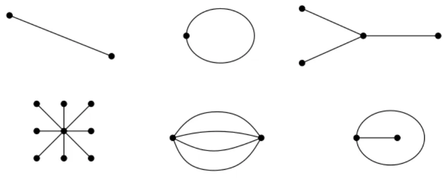
Figure 4.2: Even though the graphs are not isomorphic, the corresponding topological spaces may be homeomorphic due to useless vertices. The example graphs map intoR², and are all homeomorphic to a circle.

Figure 4.3: These topological graphs map into subsets ofR² that are not homeomorphic to each other.

isomorphisms. Let a topological graph² be a graph for which every vertex corresponds to a point in X and every edge corresponds to a continuous, injective (one-to-one) function, τ : [0,1] → X. The image of τ connects the points in X that correspond to the endpoints (vertices) of the edge. The images of diﬀerent edge functions are not allowed to intersect, except at vertices. Recall from graph theory that two graphs,G1(V1, E1) and G2(V2, E2), are called isomorphic if there exists a bijective mapping,f :V1 →V2 such that there is an edge betweenv1 and v₁^′ in G1, if and only if there exists an edge between f(v1) andf(v₁^′) in G2.

The bijective mapping used in the graph isomorphism can be extended to produce a homeomorphism. Each edge in E1 is mapped continuously to its corresponding edge in E2. The mappings nicely coincide at the vertices. Now you should see that two topological graphs are homeomorphic if they are isomorphic under the standard deﬁnition from graph theory.³ What if the graphs are not isomorphic? There is still a chance that the topological graphs may be homeomorphic, as shown in Figure 4.2. The problem is that there appear to be “useless”

vertices in the graph. By removing vertices of degree two that can be deleted without aﬀecting the connectivity of the graph, the problem is ﬁxed. In this case,

2In topology this is called a 1-complex [439].

3Technically, the images of the topological graphs, as subspaces ofX, are homeomorphic, not the graphs themselves.

(8)

graphs that are not isomorphic produce topological graphs that are not homeomorphic. This allows many distinct, interesting topological spaces to be constructed.

A few are shown in Figure 4.3.

4.1.2 Manifolds

In motion planning, efforts are made to ensure that the resulting configuration space has nice properties that reflect the true structure of the space of transformations. One important kind of topological space, which is general enough to include most of the configuration spaces considered in Part II, is called a manifold. Intu- itively, a manifold can be considered as a “nice” topological space that behaves at every point like our intuitive notion of a surface.

Manifold definition A topological space M ⊆ R^m is a manifold⁴ if for every x∈M, an open set O ⊂M exists such that: 1) x∈O, 2) O is homeomorphic to Rⁿ, and 3) n is ﬁxed for all x ∈ M. The ﬁxed n is referred to as the dimension of the manifold, M. The second condition is the most important. It states that in the vicinity of any point, x ∈ M, the space behaves just like it would in the vicinity of any point y ∈ Rⁿ; intuitively, the set of directions that one can move appears the same in either case. Several simple examples that may or may not be manifolds are shown in Figure 4.4.

One natural consequence of the deﬁnitions is that m≥n. According to Whit- ney’s embedding theorem [449],m≤2n+1. In other words,R²ⁿ⁺¹is “big enough”

to hold anyn-dimensional manifold.⁵ Technically, it is said that then-dimensional manifoldM isembeddedinR^m, which means that an injective mapping exists from M to R^m (if it is not injective, then the topology ofM could change).

As it stands, it is impossible for a manifold to include its boundary points because they are not contained in open sets. A manifold with boundary can be deﬁned requiring that the neighborhood of each boundary point of M is homeomorphic to a half-space of dimensionn (which was deﬁned for n= 2 and n= 3 in Section 3.1) and that the interior points must be homeomorphic toRⁿ.

The presentation now turns to ways of constructing some manifolds that frequently appear in motion planning. It is important to keep in mind that two

4Manifolds that are not subsets ofR^mmay also be defined. This requires thatMis a Hausdorff space and is second countable, which means that there is a countable number of open sets from which any other open set can be constructed by taking a union of some of them. These conditions are automatically satisfied when assuming M ⊆R^m; thus, it avoids these extra complications and is still general enough for our purposes. Some authors use the termmanifoldto refer to a smooth manifold. This requires the definition of a smooth structure, and the homeomorphism is replaced by diffeomorphism. This extra structure is not needed here but will be introduced when it is needed in Section 8.3.

5One variant of the theorem is that for smooth manifolds, R²ⁿ is sufficient. This bound is tight becauseRPⁿ(n-dimensional projective space, which will be introduced later in this section), cannot be embedded inR²ⁿ⁻¹.

(9)

Yes

No Yes

Yes

Yes No

Figure 4.4: Some subsets ofR² that may or may not be manifolds. For the three that are not, the point that prevents them from being manifolds is indicated.

manifolds will be considered equivalent if they are homeomorphic (recall the donut and coﬀee cup).

Cartesian products There is a convenient way to construct new topological spaces from existing ones. Suppose that X and Y are topological spaces. The Cartesian product, X × Y, deﬁnes a new topological space as follows. Every x ∈ X and y ∈ Y generates a point (x, y) in X ×Y. Each open set in X ×Y is formed by taking the Cartesian product of one open set from X and one from Y. Exactly one open set exists in X ×Y for every pair of open sets that can be formed by taking one fromX and one fromY. Furthermore, these new open sets are used as a basis for forming the remaining open sets of X×Y by allowing any unions and ﬁnite intersections of them.

A familiar example of a Cartesian product isR×R, which is equivalent toR². In general,Rⁿ is equivalent toR×Rⁿ⁻¹. The Cartesian product can be taken over many spaces at once. For example, R×R× · · · ×R = Rⁿ. In the coming text, many important manifolds will be constructed via Cartesian products.

1D manifolds The set Rof reals is the most obvious example of a 1D manifold because R certainly looks like (via homeomorphism) R in the vicinity of every point. The range can be restricted to the unit interval to yield the manifold (0,1) because they are homeomorphic (recall Example 4.5).

Another 1D manifold, which is not homeomorphic to (0,1), is a circle, S¹. In this caseR^m =R², and let

S¹ ={(x, y)∈R² |x²+y² = 1}. (4.5) If you are thinking like a topologist, it should appear that this particular circle is not important because there are numerous ways to deﬁne manifolds that are

(10)

homeomorphic to S¹. For any manifold that is homeomorphic to S¹, we will sometimes say that the manifold is S¹, just represented in a diﬀerent way. Also, S¹ will be called a circle, but this is meant only in the topological sense; it only needs to be homeomorphic to the circle that we learned about in high school geometry. Also, when referring to R, we might instead substitute (0,1) without any trouble. The alternative representations of a manifold can be considered as changingparameterizations, which are formally introduced in Section 8.3.2.

Identifications A convenient way to representS¹ is obtained byidentification, which is a general method of declaring that some points of a space are identical, even though they originally were distinct.⁶ For a topological space X, let X/∼ denote that X has been redefined through some form of identification. The open sets of X become redefined. Using identification, S¹ can be defined as [0,1]/∼, in which the identification declares that 0 and 1 are equivalent, denoted as 0∼1.

This has the eﬀect of “gluing” the ends of the interval together, forming a closed loop. To see the homeomorphism that makes this possible, use polar coordinates to obtain θ 7→ (cos 2πθ,sin 2πθ). You should already be familiar with 0 and 2π leading to the same point in polar coordinates; here they are just normalized to 0 and 1. Letting θ run from 0 up to 1, and then “wrapping around” to 0 is a convenient way to representS¹ because it does not need to be curved as in (4.5).

It might appear that identifications are cheating because the definition of a manifold requires it to be a subset ofR^m. This is not a problem because Whitney’s theorem, as mentioned previously, states that anyn-dimensional manifold can be embedded in R²ⁿ⁺¹. The identifications just reduce the number of dimensions needed for visualization. They are also convenient in the implementation of motion planning algorithms.

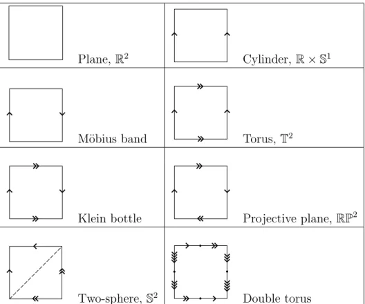
2D manifolds Many important, 2D manifolds can be defined by applying the Cartesian product to 1D manifolds. The 2D manifoldR² is formed byR×R. The product R×S¹ defines a manifold that is equivalent to an infinite cylinder. The productS¹×S¹ is a manifold that is equivalent to a torus (the surface of a donut).

Can any other 2D manifolds be defined? See Figure 4.5. The identification idea can be applied to generate several new manifolds. Start with an open square M = (0,1)×(0,1), which is homeomorphic toR². Let (x, y) denote a point in the plane. A flat cylinder is obtained by making the identification (0, y) ∼ (1, y) for ally∈(0,1) and adding all of these points to M. The result is depicted in Figure 4.5 by drawing arrows where the identification occurs.

A Möbius band can be constructed by taking a strip of paper and connecting the ends after making a 180-degree twist. This result is not homeomorphic to the cylinder. The Möbius band can also be constructed by putting the twist into the identification, as (0, y)∼ (1,1−y) for all y ∈ (0,1). In this case, the arrows are drawn in opposite directions. The Möbius band has the famous properties that

6This is usually defined more formally and called aquotient topology.

(11)

Plane, R² Cylinder,R×S¹

M¨obius band Torus, T²

Klein bottle Projective plane, RP²

Two-sphere, S² Double torus

Figure 4.5: Some 2D manifolds that can be obtained by identifying pairs of points along the boundary of a square region.

it has only one side (trace along the paper strip with a pencil, and you will visit both sides of the paper) and is nonorientable (if you try to draw it in the plane, without using identiﬁcation tricks, it will always have a twist).

For all of the cases so far, there has been a boundary to the set. The next few manifolds will not even have a boundary, even though they may be bounded. If you were to live in one of them, it means that you could walk forever along any trajectory and never encounter the edge of your universe. It might seem like our physical universe is unbounded, but it would only be an illusion. Furthermore, there are several distinct possibilities for the universe that are not homeomorphic to each other. In higher dimensions, such possibilities are the subject of cosmology, which is a branch of astrophysics that uses topology to characterize the structure of our universe.

A torus can be constructed by performing identifications of the form (0, y) ∼ (1, y), which was done for the cylinder, and also (x,0)∼(x,1), which identifies the top and bottom. Note that the point (0,0) must be included and is identified with three other points. Double arrows are used in Figure 4.5 to indicate the top and bottom identification. All of the identification points must be added to M. Note that there are no twists. A funny interpretation of the resultingflat torus is as the universe appears for a spacecraft in some 1980s-style Asteroids-like video games.

(12)

The spaceship flies off of the screen in one direction and appears somewhere else, as prescribed by the identification.

Two interesting manifolds can be made by adding twists. Consider performing all of the identifications that were made for the torus, except put a twist in the side identification, as was done for the Möbius band. This yields a fascinating manifold called the Klein bottle, which can be embedded in R⁴ as a closed 2D surface in which the inside and the outside are the same! (This is in a sense similar to that of the Möbius band.) Now suppose there are twists in both the sides and the top and bottom. This results in the most bizarre manifold yet: the real projective plane, RP². This space is equivalent to the set of all lines in R³ that pass through the origin. The 3D version,RP³, happens to be one of the most important manifolds for motion planning!

LetS² denote the unit sphere, which is deﬁned as

S² ={(x, y, z)∈R³ |x²+y²+z² = 1}. (4.6) Another way to represent S² is by making the identiﬁcations shown in the last row of Figure 4.5. A dashed line is indicated where the equator might appear, if we wanted to make a distorted wall map of the earth. The poles would be at the upper left and lower right corners. The ﬁnal example shown in Figure 4.5 is a double torus, which is the surface of a two-holed donut.

Higher dimensional manifolds The construction techniques used for the 2D manifolds generalize nicely to higher dimensions. Of course,Rⁿ, is ann-dimensional manifold. Ann-dimensional torus, Tⁿ, can be made by taking a Cartesian product ofn copies of S¹. Note that S¹×S¹ 6=S². Therefore, the notation Tⁿ is used for (S¹)ⁿ. Diﬀerent kinds of n-dimensional cylinders can be made by forming a Cartesian productRⁱ×T^j for positive integersiandj such thati+j =n. Higher dimensional spheres are deﬁned as

Sⁿ={x∈Rⁿ⁺¹ | kxk= 1}, (4.7) in which kxkdenotes the Euclidean norm of x, and n is a positive integer. Many interesting spaces can be made by identifying faces of the cube (0,1)ⁿ(or even faces of a polyhedron or polytope), especially if different kinds of twists are allowed. An n-dimensional projective space can be defined in this way, for example. Lens spaces are a family of manifolds that can be constructed by identification of polyhedral faces [834].

Due to its coming importance in motion planning, more details are given on projective spaces. The standard deﬁnition of an n-dimensional real projective space RPⁿ is the set of all lines in Rⁿ⁺¹ that pass through the origin. Each line is considered as a point in RPⁿ. Using the deﬁnition of Sⁿ in (4.7), note that each of these lines in Rⁿ⁺¹ intersects Sⁿ ⊂ Rⁿ⁺¹ in exactly two places. These intersection points are called antipodal, which means that they are as far from each other as possible onSⁿ. The pair is also unique for each line. If we identify

(13)

4.1. BASIC TOPOLOGICAL CONCEPTS 139 all pairs of antipodal points ofSⁿ, a homeomorphism can be deﬁned between each line through the origin ofRⁿ⁺¹ and each antipodal pair on the sphere. This means that the resulting manifold, Sⁿ/∼, is homeomorphic to RPⁿ.

Another way to interpret the identification is that RPⁿ is just the upper half ofSⁿ, but with every equatorial point identified with its antipodal point. Thus, if you try to walk into the southern hemisphere, you will find yourself on the other side of the world walking north. It is helpful to visualize the special case of RP² and the upper half of S². Imagine warping the picture of RP² from Figure 4.5 from a square into a circular disc, with opposite points identified. The result still representsRP². The center of the disc can now be lifted out of the plane to form the upper half of S².

4.1.3 Paths and Connectivity

Central to motion planning is determining whether one part of a space is reachable from another. In Chapter 2, one state was reached from another by applying a sequence of actions. For motion planning, the analog to this is connecting one point in the conﬁguration space to another by a continuous path. Graph connectivity is important in the discrete planning case. An analog to this for topological spaces is presented in this section.

Paths LetX be a topological space, which for our purposes will also be a manifold. A path is a continuous function, τ : [0,1] → X. Alternatively, R may be used for the domain of τ. Keep in mind that a path is a function, not a set of points. Each point along the path is given byτ(s) for somes∈[0,1]. This makes it appear as a nice generalization to the sequence of states visited when a plan from Chapter 2 is applied. Recall that there, a countable set of stages was deﬁned, and the states visited could be represented as x1, x2, . . .. In the current setting τ(s) is used, in which s replaces the stage index. To make the connection clearer, we could use xinstead of τ to obtain x(s) for each s∈[0,1].

Connected vs. path connected A topological spaceX is said to beconnected if it cannot be represented as the union of two disjoint, nonempty, open sets. While this deﬁnition is rather elegant and general, if X is connected, it does not imply that a path exists between any pair of points in X thanks to crazy examples like the topologist’s sine curve:

X ={(x, y)∈R² |x= 0 or y= sin(1/x)}. (4.8) Consider plotting X. The sin(1/x) part creates oscillations near the y-axis in which the frequency tends to inﬁnity. After union is taken with the y-axis, this space is connected, but there is no path that reaches they-axis from the sine curve.

How can we avoid such problems? The standard way to fix this is to use the path definition directly in the definition of connectedness. A topological space X is said to be path connected if for all x1, x2 ∈ X, there exists a path τ such that

(14)

t= 0

t= 1 t= 1/3 t= 2/3

t= 0

t= 1

(a) (b)

Figure 4.6: (a) Homotopy continuously warps one path into another. (b) The image of the path cannot be continuously warped over a hole in R² because it causes a discontinuity. In this case, the two paths are not homotopic.

τ(0) =x1 and τ(1) =x2. It can be shown that ifX is path connected, then it is also connected in the sense deﬁned previously.

Another way to fix it is to make restrictions on the kinds of topological spaces that will be considered. This approach will be taken here by assuming that all topological spaces are manifolds. In this case, no strange things like (4.8) can happen,⁷ and the definitions of connected and path connected coincide [451]. Therefore, we will just say a space isconnected. However, it is important to remember that this definition of connected is sometimes inadequate, and one should really say thatX ispath connected.

Simply connected Now that the notion of connectedness has been established, the next step is to express diﬀerent kinds of connectivity. This may be done by using the notion of homotopy, which can intuitively be considered as a way to continuously “warp” or “morph” one path into another, as depicted in Figure 4.6a.

Two pathsτ₁ and τ₂ are calledhomotopic (with endpoints ﬁxed) if there exists a continuous functionh: [0,1]×[0,1]→X for which the following four conditions are met:

1. (Start with first path) h(s,0) =τ1(s) for all s∈[0,1] . 2. (End with second path) h(s,1) =τ₂(s) for all s∈[0,1] . 3. (Hold starting point fixed) h(0, t) =h(0,0) for allt ∈[0,1] . 4. (Hold ending point fixed) h(1, t) = h(1,0) for allt ∈[0,1] .

7The topologist’s sine curve is not a manifold because all open sets that contain the point (0,0) contain some of the points from the sine curve. These open sets are not homeomorphic to R.

(15)

4.1. BASIC TOPOLOGICAL CONCEPTS 141 The parameter t can be interpreted as a knob that is turned to gradually deform the path fromτ₁ intoτ₂. The ﬁrst two conditions indicate that t= 0 yields τ₁ and t= 1 yieldsτ2, respectively. The remaining two conditions indicate that the path endpoints are held ﬁxed.

During the warping process, the path image cannot make a discontinuous jump.

InR², this prevents it from moving over holes, such as the one shown in Figure 4.6b.

The key to preventing homotopy from jumping over some holes is that hmust be continuous. In higher dimensions, however, there are many diﬀerent kinds of holes.

For the case of R³, for example, suppose the space is like a block of Swiss cheese that contains air bubbles. Homotopy can go around the air bubbles, but it cannot pass through a hole that is drilled through the entire block of cheese. Air bubbles and other kinds of holes that appear in higher dimensions can be characterized by generalizing homotopy to the warping of higher dimensional surfaces, as opposed to paths [439].

It is straightforward to show that homotopy deﬁnes an equivalence relation on the set of all paths from some x1 ∈ X to some x2 ∈ X. The resulting notion of “equivalent paths” appears frequently in motion planning, control theory, and many other contexts. Suppose thatX is path connected. If all paths fall into the same equivalence class, then X is called simply connected; otherwise, X is called multiply connected.

Groups The equivalence relation induced by homotopy starts to enter the realm of algebraic topology, which is a branch of mathematics that characterizes the structure of topological spaces in terms of algebraic objects, such as groups. These resulting groups have important implications for motion planning. Therefore, we give a brief overview. First, the notion of a group must be precisely deﬁned. A group is a set, G, together with a binary operation, ◦, such that the following group axioms are satisﬁed:

1. (Closure) For any a, b∈G, the product a◦b∈G.

2. (Associativity) For alla, b, c∈G, (a◦b)◦c=a◦(b◦c). Hence, parentheses are not needed, and the product may be written as a◦b◦c.

3. (Identity) There is an element e ∈G, called the identity, such that for all a ∈G, e◦a=a and a◦e =a.

4. (Inverse) For every element a ∈ G, there is an element a⁻¹, called the inverse of a, for whicha◦a⁻¹ =e and a⁻¹◦a=e.

Here are some examples.

Example 4.7 (Simple Examples of Groups) The set of integersZ is a group with respect to addition. The identity is 0, and the inverse of eachiis−i. The set Q\0 of rational numbers with 0 removed is a group with respect to multiplication.

The identity is 1, and the inverse of every element, q, is 1/q (0 was removed to

(16)

avoid division by zero).

An important property, which only some groups possess, is commutativity:

a◦b = b ◦a for any a, b ∈ G. The group in this case is called commutative or Abelian. We will encounter examples of both kinds of groups, both commutative and noncommutative. An example of a commutative group is vector addition over Rⁿ. The set of all 3D rotations is an example of a noncommutative group.

The fundamental group Now an interesting group will be constructed from the space of paths and the equivalence relation obtained by homotopy. Thefunda- mental group, π1(X) (or first homotopy group), is associated with any topological space, X. Let a (continuous) path for which f(0) = f(1) be called a loop. Let some x_b ∈ X be designated as a base point. For some arbitrary but fixed base point, xb, consider the set of all loops such that f(0) = f(1) = xb. This can be made into a group by defining the following binary operation. Let τ1 : [0,1]→X and τ2 : [0,1] → X be two loop paths with the same base point. Their product τ =τ1 ◦τ2 is defined as

τ(t) =

τ1(2t) if t∈[0,1/2)

τ2(2t−1) if t∈[1/2,1]. (4.9) This results in a continuous loop path because τ₁ terminates atx_b, and τ₂ begins atxb. In a sense, the two paths are concatenated end-to-end.

Suppose now that the equivalence relation induced by homotopy is applied to the set of all loop paths through a ﬁxed point, x_b. It will no longer be important which particular path was chosen from a class; any representative may be used.

The equivalence relation also applies when the set of loops is interpreted as a group. The group operation actually occurs over the set of equivalences of paths.

Consider what happens when two paths from diﬀerent equivalence classes are concatenated using ◦. Is the resulting path homotopic to either of the ﬁrst two?

Is the resulting path homotopic if the original two are from the same homotopy class? The answers in general areno andno, respectively. The fundamental group describes how the equivalence classes of paths are related and characterizes the connectivity of X. Since fundamental groups are based on paths, there is a nice connection to motion planning.

Example 4.8 (A Simply Connected Space) Suppose that a topological space X is simply connected. In this case, all loop paths from a base pointx_b are homotopic, resulting in one equivalence class. The result is π1(X) =1^G, which is the

group that consists of only the identity element.

Example 4.9 (The Fundamental Group of S¹) Suppose X = S¹. In this case, there is an equivalence class of paths for each i ∈ Z, the set of integers.

(17)

1

1 1

1 2

2

1

2 1 2

(a) (b) (c)

Figure 4.7: An illustration of why π1(RP²) = Z₂. The integers 1 and 2 indicate precisely where a path continues when it reaches the boundary. (a) Two paths are shown that are not equivalent. (b) A path that winds around twice is shown. (c) This is homotopic to a loop path that does not wind around at all. Eventually, the part of the path that appears at the bottom is pulled through the top. It ﬁnally shrinks into an arbitrarily small loop.

Ifi >0, then it means that the path winds itimes around S¹ in the counterclockwise direction and then returns tox_b. Ifi <0, then the path winds arounditimes in the clockwise direction. Ifi= 0, then the path is equivalent to one that remains atxb. The fundamental group is Z, with respect to the operation of addition. If τ1 travelsi1 times counterclockwise, andτ2 travels i2 times counterclockwise, then τ =τ₁◦τ₂ belongs to the class of loops that travel around i₁+i₂ times counterclockwise. Consider additive inverses. If a path travels seven times aroundS¹, and it is combined with a path that travels seven times in the opposite direction, the result is homotopic to a path that remains atxb. Thus, π1(S¹) = Z.

Example 4.10 (The Fundamental Group of Tⁿ) For the torus,π1(Tⁿ) = Zⁿ, in which theith component ofZⁿ corresponds to the number of times a loop path wraps around theith component of Tⁿ. This makes intuitive sense because Tⁿ is just the Cartesian product ofn circles. The fundamental group Zⁿ is obtained by starting with a simply connected subset of the plane and drilling out n disjoint, bounded holes. This situation arises frequently when a mobile robot must avoid

collision withn disjoint obstacles in the plane.

By now it seems that the fundamental group simply keeps track of how many times a path travels around holes. This next example yields some very bizarre behavior that helps to illustrate some of the interesting structure that arises in algebraic topology.

(18)

Example 4.11 (The Fundamental Group of RP²) Suppose X = RP², the projective plane. In this case, there are only two equivalence classes on the space of loop paths. All paths that “wrap around” an even number of times are homotopic.

Likewise, all paths that wrap around an odd number of times are homotopic. This strange behavior is illustrated in Figure 4.7. The resulting fundamental group therefore has only two elements: π1(RP²) = Z₂, the cyclic group of order 2, which corresponds to addition mod 2. This makes intuitive sense because the group keeps track of whether a sum of integers is odd or even, which in this application corresponds to the total number of traversals over the square representation of RP². The fundamental group is the same for RP³, which arises in Section 4.2.2 because it is homeomorphic to the set of 3D rotations. Thus, there are surprisingly

only two path classes for the set of 3D rotations.

Unfortunately, two topological spaces may have the same fundamental group even if the spaces are not homeomorphic. For example, Z is the fundamental group of S¹, the cylinder, R×S¹, and the Möbius band. In the last case, the fundamental group does not indicate that there is a “twist” in the space. Another problem is that spaces with interesting connectivity may be declared as simply connected. The fundamental group of the sphere S² is just 1G, the same as for R². Try envisioning loop paths on the sphere; it can be seen that they all fall into one equivalence class. Hence,S² is simply connected. The fundamental group also neglects bubbles inR³ because the homotopy can warp paths around them. Some of these troubles can be fixed by defining second-order homotopy groups. For example, a continuous function, [0,1]×[0,1] → X, of two variables can be used instead of a path. The resulting homotopy generates a kind of sheet or surface that can be warped through the space, to yield a homotopy group π2(X) that wraps around bubbles in R³. This idea can be extended beyond two dimensions to detect many different kinds of holes in higher dimensional spaces. This leads to the higher order homotopy groups. A stronger concept than simply connected for a space is that its homotopy groups of all orders are equal to the identity group.

This prevents all kinds of holes from occurring and implies that a space, X, is contractible, which means a kind of homotopy can be constructed that shrinks X to a point [439]. In the plane, the notions ofcontractible andsimply connectedare equivalent; however, in higher dimensional spaces, such as those arising in motion planning, the term contractible should be used to indicate that the space has no interior obstacles (holes).

An alternative to basing groups on homotopy is to derive them usinghomology, which is based on the structure of cell complexes instead of homotopy mappings.

This subject is much more complicated to present, but it is more powerful for proving theorems in topology. See the literature overview at the end of the chapter for suggested further reading on algebraic topology.

(19)

4.2. DEFINING THE CONFIGURATION SPACE 145

4.2 Defining the Configuration Space

This section defines the manifolds that arise from the transformations of Chapter 3. If the robot has n degrees of freedom, the set of transformations is usually a manifold of dimension n. This manifold is called the configuration space of the robot, and its name is often shortened to C-space. In this book, the C-space may be considered as a special state space. To solve a motion planning problem, algorithms must conduct a search in the C-space. The C-space provides a powerful abstraction that converts the complicated models and transformations of Chapter 3 into the general problem of computing a path that traverses a manifold. By developing algorithms directly for this purpose, they apply to a wide variety of different kinds of robots and transformations. In Section 4.3 the problem will be complicated by bringing obstacles into the configuration space, but in Section 4.2 there will be no obstacles.

4.2.1 2D Rigid Bodies: SE(2)

Section 3.2.2 expressed how to transform a rigid body in R² by a homogeneous transformation matrix, T, given by (3.35). The task in this chapter is to characterize the set of all possible rigid-body transformations. Which manifold will this be? Here is the answer and brief explanation. Since any x_t, y_t ∈ R can be selected for translation, this alone yields a manifoldM1 =R². Independently, any rotation, θ ∈[0,2π), can be applied. Since 2π yields the same rotation as 0, they can be identiﬁed, which makes the set of 2D rotations into a manifold, M2 =S¹. To obtain the manifold that corresponds to all rigid-body motions, simply take C =M₁×M₂ =R²×S¹. The answer to the question is that the C-space is a kind of cylinder.

Now we give a more detailed technical argument. The main purpose is that such a simple, intuitive argument will not work for the 3D case. Our approach is to introduce some of the technical machinery here for the 2D case, which is easier to understand, and then extend it to the 3D case in Section 4.2.2.

Matrix groups The ﬁrst step is to consider the set of transformations as a group, in addition to a topological space.⁸ We now derive several important groups from sets of matrices, ultimately leading to SO(n), the group of n×n rotation matrices, which is very important for motion planning. The set of all nonsingular n×n real-valued matrices is called the general linear group, denoted by GL(n), with respect to matrix multiplication. Each matrix A ∈ GL(n) has an inverse A⁻¹ ∈ GL(n), which when multiplied yields the identity matrix, AA⁻¹ = I. The

8The groups considered in this section are actually Lie groups because they are smooth manifolds [63]. We will not use that name here, however, because the notion of a smooth structure has not yet been defined. Readers familiar with Lie groups, however, will recognize most of the coming concepts. Some details on Lie groups appear later in Sections 15.4.3 and 15.5.1.

(20)

matrices must be nonsingular for the same reason that 0 was removed fromQ. The analog of division by zero for matrix algebra is the inability to invert a singular matrix.

Many interesting groups can be formed from one group,G1, by removing some elements to obtain a subgroup, G2. To be a subgroup, G2 must be a subset of G1 and satisfy the group axioms. We will arrive at the set of rotation matrices by constructing subgroups. One important subgroup of GL(n) is the orthogonal group, O(n), which is the set of all matrices A ∈ GL(n) for which AA^T = I, in which A^T denotes the matrix transpose of A. These matrices have orthogonal columns (the inner product of any pair is zero) and the determinant is always 1 or

−1. Thus, note thatAA^T takes the inner product of every pair of columns. If the columns are diﬀerent, the result must be 0; if they are the same, the result is 1 because AA^T =I. The special orthogonal group, SO(n), is the subgroup of O(n) in which every matrix has determinant 1. Another name for SO(n) is the group of n-dimensional rotation matrices.

A chain of groups, SO(n) ≤ O(n) ≤ GL(n), has been described in which ≤ denotes “a subgroup of.” Each group can also be considered as a topological space.

The set of alln×n matrices (which is not a group with respect to multiplication) with real-valued entries is homeomorphic to Rⁿ² because n² entries in the matrix can be independently chosen. For GL(n), singular matrices are removed, but an n²-dimensional manifold is nevertheless obtained. ForO(n), the expressionAA^T = I corresponds to n² algebraic equations that have to be satisﬁed. This should substantially drop the dimension. Note, however, that many of the equations are redundant (pick your favorite value for n, multiply the matrices, and see what happens). There are only (ⁿ₂) ways (pairwise combinations) to take the inner product of pairs of columns, and there aren equations that require the magnitude of each column to be 1. This yields a total of n(n+ 1)/2 independent equations.

Each independent equation drops the manifold dimension by one, and the resulting dimension ofO(n) isn²−n(n+ 1)/2 =n(n−1)/2, which is easily remembered as (ⁿ₂). To obtain SO(n), the constraint detA= 1 is added, which eliminates exactly half of the elements ofO(n) but keeps the dimension the same.

Example 4.12 (Matrix Subgroups) It is helpful to illustrate the concepts for n= 2. The set of all 2×2 matrices is

a b c d

a, b, c, d∈R

, (4.10)

which is homeomorphic to R⁴. The group GL(2) is formed from the set of all nonsingular 2×2 matrices, which introduces the constraint thatad−bc6= 0. The set of singular matrices forms a 3D manifold with boundary in R⁴, but all other elements ofR⁴ are in GL(2); therefore, GL(2) is a 4D manifold.

Next, the constraintAA^T =I is enforced to obtain O(2). This becomes a b

c d

a c b d

= 1 0

0 1

, (4.11)

(21)

4.2. DEFINING THE CONFIGURATION SPACE 147 which directly yields four algebraic equations:

a²+b² = 1 (4.12)

ac+bd= 0 (4.13)

ca+db= 0 (4.14)

c²+d² = 1. (4.15)

Note that (4.14) is redundant. There are two kinds of equations. One equation, given by (4.13), forces the inner product of the columns to be 0. There is only one because (ⁿ₂) = 1 forn= 2. Two other constraints, (4.12) and (4.15), force the rows to be unit vectors. There are two becausen= 2. The resulting dimension of the manifold is (ⁿ₂) = 1 because we started withR⁴ and lost three dimensions from (4.12), (4.13), and (4.15). What does this manifold look like? Imagine that there are two diﬀerent two-dimensional unit vectors, (a, b) and (c, d). Any value can be chosen for (a, b) as long as a²+b² = 1. This looks like S¹, but the inner product of (a, b) and (c, d) must also be 0. Therefore, for each value of (a, b), there are two choices for c and d: 1) c = b and d = −a, or 2) c = −b and d = a. It appears that there are two circles! The manifold is S¹⊔S¹, in which ⊔ denotes the union of disjoint sets. Note that this manifold is not connected because no path exists from one circle to the other.

The ﬁnal step is to require that detA=ad−bc= 1, to obtain SO(2), the set of all 2D rotation matrices. Without this condition, there would be matrices that produce a rotated mirror image of the rigid body. The constraint simply forces the choice forcanddto be c=−band a=d. This throws away one of the circles fromO(2), to obtain a single circle for SO(2). We have ﬁnally obtained what you already knew: SO(2) is homeomorphic to S¹. The circle can be parameterized using polar coordinates to obtain the standard 2D rotation matrix, (3.31), given

in Section 3.2.2.

Special Euclidean group Now that the group of rotations, SO(n), is characterized, the next step is to allow both rotations and translations. This corresponds to the set of all (n+ 1)×(n+ 1) transformation matrices of the form

R v 0 1

R∈SO(n) and v ∈Rⁿ

. (4.16)

This should look like a generalization of (3.52) and (3.56), which were for n = 2 and n = 3, respectively. The R part of the matrix achieves rotation of an n- dimensional body in Rⁿ, and the v part achieves translation of the same body.

The result is a group, SE(n), which is called the special Euclidean group. As a topological space, SE(n) is homeomorphic to Rⁿ×SO(n), because the rotation matrix and translation vectors may be chosen independently. In the case ofn = 2, this means SE(2) is homeomorphic to R² × S¹, which veriﬁes what was stated

(22)

qI

qG

Figure 4.8: A planning algorithm may have to cross the identiﬁcation boundary to ﬁnd a solution path.

at the beginning of this section. Thus, the C-space of a 2D rigid body that can translate and rotate in the plane is

C =R²×S¹. (4.17)

To be more precise, ∼= should be used in the place of = to indicate thatC could be any space homeomorphic to R² × S¹; however, this notation will mostly be avoided.

Interpreting the C-space It is important to consider the topological implications of C. Since S¹ is multiply connected, R× S¹ and R² ×S¹ are multiply connected. It is difficult to visualize C because it is a 3D manifold; however, there is a nice interpretation using identification. Start with the open unit cube, (0,1)³ ⊂ R³. Include the boundary points of the form (x, y,0) and (x, y,1), and make the identification (x, y,0) ∼ (x, y,1) for all x, y ∈ (0,1). This means that when traveling in the x and y directions, there is a “frontier” to the C-space;

however, traveling in thez direction causes a wraparound.

It is very important for a motion planning algorithm to understand that this wraparound exists. For example, consider R×S¹ because it is easier to visualize.

Imagine a path planning problem for which C = R×S¹, as depicted in Figure 4.8. Suppose the top and bottom are identified to make a cylinder, and there is an obstacle across the middle. Suppose the task is to find a path fromqI toqG. If the top and bottom were not identified, then it would not be possible to connect qI to qG; however, if the algorithm realizes it was given a cylinder, the task is straightforward. In general, it is very important to understand the topology ofC; otherwise, potential solutions will be lost.

The next section addressesSE(n) forn= 3. The main diﬃculty is determining the topology ofSO(3). At least we do not have to consider n >3 in this book.

4.2.2 3D Rigid Bodies: SE(3)

One might expect that deﬁningC for a 3D rigid body is an obvious extension of the 2D case; however, 3D rotations are signiﬁcantly more complicated. The resulting

(23)

4.2. DEFINING THE CONFIGURATION SPACE 149 C-space will be a six-dimensional manifold,C =R³×RP³. Three dimensions come from translation and three more come from rotation.

The main quest in this section is to determine the topology ofSO(3). In Section 3.2.3, yaw, pitch, and roll were used to generate rotation matrices. These angles are convenient for visualization, performing transformations in software, and also for deriving the DH parameters. However, these were concerned with applying a single rotation, whereas the current problem is to characterize the set of all rotations. It is possible to use α, β, and γ to parameterize the set of rotations, but it causes serious troubles. There are some cases in which nonzero angles yield the identity rotation matrix, which is equivalent to α = β = γ = 0. There are also cases in which a continuum of values for yaw, pitch, and roll angles yield the same rotation matrix. These problems destroy the topology, which causes both theoretical and practical diﬃculties in motion planning.

Consider applying the matrix group concepts from Section 4.2.1. The general linear group GL(3) is homeomorphic to R⁹. The orthogonal group, O(3), is de- termined by imposing the constraint AA^T = I. There are (³₂) = 3 independent equations that require distinct columns to be orthogonal, and three independent equations that force the magnitude of each column to be 1. This means thatO(3) has three dimensions, which matches our intuition since there were three rotation parameters in Section 3.2.3. To obtain SO(3), the last constraint, detA = 1, is added. Recall from Example 4.12 that SO(2) consists of two circles, and the constraint detA = 1 selects one of them. In the case of O(3), there are two three-spheres, S³⊔S³, and detA = 1 selects one of them. However, there is one additional complication: Antipodal points on these spheres generate the same rotation matrix. This will be seen shortly when quaternions are used to parameterize SO(3).

Using complex numbers to represent SO(2) Before introducing quaternions to parameterize 3D rotations, consider using complex numbers to parameterize 2D rotations. Let the termunit complex numberrefer to any complex number, a+bi, for which a²+b² = 1.

The set of all unit complex numbers forms a group under multiplication. It will be seen that it is “the same” group as SO(2). This idea needs to be made more precise. Two groups, Gand H, are considered “the same” if they are isomorphic, which means that there exists a bijective function f : G → H such that for all a, b∈G,f(a)◦f(b) =f(a◦b). This means that we can perform some calculations inG, map the result toH, perform more calculations, and map back toGwithout any trouble. The setsG and H are just two alternative ways to express the same group.

The unit complex numbers andSO(2) are isomorphic. To see this clearly, recall that complex numbers can be represented in polar form as reîθ; a unit complex number is simply eîθ. A bijective mapping can be made between 2D rotation matrices and unit complex numbers by lettingeîθ correspond to the rotation matrix (3.31).

(24)

If complex numbers are used to represent rotations, it is important that they behave algebraically in the same way. If two rotations are combined, the matrices are multiplied. The equivalent operation is multiplication of complex numbers.

Suppose that a 2D robot is rotated byθ1, followed byθ2. In polar form, the complex numbers are multiplied to yield eîθ¹eîθ² = eî(θ¹^+θ²⁾, which clearly represents a rotation ofθ1+θ2. If the unit complex number is represented in Cartesian form, then the rotations corresponding to a₁ +b₁i and a₂+b₂i are combined to obtain (a1a2−b1b2) + (a1b2+a2b1)i. Note that here we have not used complex numbers to express the solution to a polynomial equation, which is their more popular use; we simply borrowed their nice algebraic properties. At any time, a complex number a+bi can be converted into the equivalent rotation matrix

R(a, b) =

a −b b a

. (4.18)

Recall that only one independent parameter needs to be speciﬁed because a² + b² = 1. Hence, it appears that the set of unit complex numbers is the same manifold asSO(2), which is the circle S¹ (recall, that “same” means in the sense of homeomorphism).

Quaternions The manner in which complex numbers were used to represent 2D rotations will now be adapted to using quaternions to represent 3D rotations. Let Hrepresent the set ofquaternions, in which each quaternion,h∈H, is represented ash=a+bi+cj+dk, anda, b, c, d∈R. A quaternion can be considered as a four- dimensional vector. The symbolsi,j, andk are used to denote three “imaginary”

components of the quaternion. The following relationships are deﬁned: i² =j² = k² = ijk = −1, from which it follows that ij = k, jk = i, and ki = j. Using these, multiplication of two quaternions, h1 = a1 +b1i +c1j +d1k and h2 = a2+b2i+c2j+d2k, can be derived to obtainh1·h2 =a3+b3i+c3j+d3k, in which

a3 =a1a2−b1b2 −c1c2−d1d2

b3 =a1b2+a2b1+c1d2−c2d1

c3 =a1c2+a2c1+b2d1−b1d2

d₃ =a₁d₂+a₂d₁ +b₁c₂−b₂c₁.

(4.19)

Using this operation, it can be shown thatHis a group with respect to quaternion multiplication. Note, however, that the multiplication is not commutative! This is also true of 3D rotations; there must be a good reason.

For convenience, quaternion multiplication can be expressed in terms of vector multiplications, a dot product, and a cross product. Let v = [b c d] be a three- dimensional vector that represents the final three quaternion components. The first component of h1 ·h2 is a1a2−v1·v2. The final three components are given by the three-dimensional vectora1v2+a2v1+v1×v2.

In the same way thatunitcomplex numbers were needed forSO(2),unit quaternions are needed for SO(3), which means that H is restricted to quaternions for