Chapter 6
Dynamic Programming
We began our study of algorithmic techniques with greedy algorithms, which in some sense form the most natural approach to algorithm design. Faced with a new computational problem, we’ve seen that it’s not hard to propose multiple possible greedy algorithms; the challenge is then to determine whether any of these algorithms provides a correct solution to the problem in all cases.
The problems we saw in Chapter 4 were all unified by the fact that, in the end, there really was a greedy algorithm that worked. Unfortunately, this is far from being true in general; for most of the problems that one encounters, the real difficulty is not in determining which of several greedy strategies is the right one, but in the fact that there isnonatural greedy algorithm that works.
For such problems, it is important to have other approaches at hand. Divide and conquer can sometimes serve as an alternative approach, but the versions of divide and conquer that we saw in the previous chapter are often not strong enough to reduce exponential brute-force search down to polynomial time.
Rather, as we noted in Chapter 5, the applications there tended to reduce a running time that was unnecessarily large, but already polynomial, down to a faster running time.
We now turn to a more powerful and subtle design technique, dynamic programming. It will be easier to say exactly what characterizes dynamic pro- gramming after we’ve seen it in action, but the basic idea is drawn from the intuition behind divide and conquer and is essentially the opposite of the greedy strategy: one implicitly explores the space of all possible solutions, by carefully decomposing things into a series of subproblems, and then build- ing up correct solutions to larger and larger subproblems. In a way, we can thus view dynamic programming as operating dangerously close to the edge of
brute-force search: although it’s systematically working through the exponen- tially large set of possible solutions to the problem, it does this without ever examining them all explicitly. It is because of this careful balancing act that dynamic programming can be a tricky technique to get used to; it typically takes a reasonable amount of practice before one is fully comfortable with it.
With this in mind, we now turn to a first example of dynamic program- ming: the Weighted Interval Scheduling Problem that we defined back in Section 1.2. We are going to develop a dynamic programming algorithm for this problem in two stages: first as a recursive procedure that closely resembles brute-force search; and then, by reinterpreting this procedure, as an iterative algorithm that works by building up solutions to larger and larger subproblems.
6.1 Weighted Interval Scheduling:
A Recursive Procedure
We have seen that a particular greedy algorithm produces an optimal solution to the Interval Scheduling Problem, where the goal is to accept as large a set of nonoverlapping intervals as possible. The Weighted Interval Scheduling Problem is a strictly more general version, in which each interval has a certain value(orweight), and we want to accept a set of maximum value.
Designing a Recursive Algorithm
Since the original Interval Scheduling Problem is simply the special case in which all values are equal to 1, we know already that most greedy algorithms will not solve this problem optimally. But even the algorithm that worked before (repeatedly choosing the interval that ends earliest) is no longer optimal in this more general setting, as the simple example in Figure 6.1 shows.
Indeed, no natural greedy algorithm is known for this problem, which is what motivates our switch to dynamic programming. As discussed above, we will begin our introduction to dynamic programming with a recursive type of algorithm for this problem, and then in the next section we’ll move to a more iterative method that is closer to the style we use in the rest of this chapter.
Index 1 2 3
Value = 1
Value = 3 Value = 1
Figure 6.1 A simple instance of weighted interval scheduling.
6.1 Weighted Interval Scheduling: A Recursive Procedure
253
We use the notation from our discussion of Interval Scheduling in Sec- tion 1.2. We havenrequests labeled 1, . . . ,n, with each requestispecifying a start timesiand a finish timefi. Each intervalinow also has avalue, orweight vi. Two intervals arecompatibleif they do not overlap. The goal of our current problem is to select a subsetS⊆ {1, . . . ,n}of mutually compatible intervals, so as to maximize the sum of the values of the selected intervals,
i∈Svi. Let’s suppose that the requests are sorted in order of nondecreasing finish time:f1≤f2≤. . .≤fn. We’ll say a requesti comesbeforea requestjifi<j.
This will be the natural left-to-right order in which we’ll consider intervals.
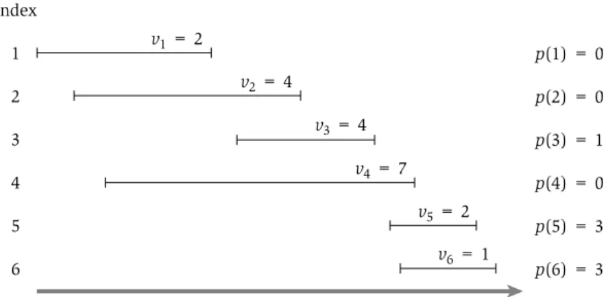
To help in talking about this order, we definep(j), for an intervalj, to be the largest index i<j such that intervals i and j are disjoint. In other words, i is the leftmost interval that ends before j begins. We define p(j)=0 if no requesti<jis disjoint from j. An example of the definition of p(j)is shown in Figure 6.2.
Now, given an instance of the Weighted Interval Scheduling Problem, let’s consider an optimal solutionO, ignoring for now that we have no idea what it is. Here’s something completely obvious that we can say aboutO: either intervaln(the last one) belongs toO, or it doesn’t. Suppose we explore both sides of this dichotomy a little further. Ifn∈O, then clearly no interval indexed strictly betweenp(n)andncan belong toO, because by the definition ofp(n), we know that intervals p(n)+1,p(n)+2, . . . ,n−1 all overlap interval n.
Moreover, ifn∈O, thenOmust include anoptimal solution to the problem consisting of requests {1, . . . ,p(n)}—for if it didn’t, we could replace O’s choice of requests from {1, . . . ,p(n)}with a better one, with no danger of overlapping requestn.
Index 1 2 3 4 5 6
p(1) = 0 p(2) = 0 p(3) = 1 p(4) = 0 p(5) = 3 p(6) = 3 v1 = 2
v3 = 4 v2 = 4
v5 = 2 v6 = 1 v4 = 7
Figure 6.2 An instance of weighted interval scheduling with the functionsp(j)defined for each intervalj.
On the other hand, ifn∈O, thenOis simply equal to the optimal solution to the problem consisting of requests {1, . . . ,n−1}. This is by completely analogous reasoning: we’re assuming thatOdoes not include requestn; so if it does not choose the optimal set of requests from {1, . . . ,n−1}, we could replace it with a better one.
All this suggests that finding the optimal solution on intervals{1, 2, . . . ,n}
involves looking at the optimal solutions of smaller problems of the form {1, 2, . . . ,j}. Thus, for any value ofjbetween 1 andn, letOjdenote the optimal solution to the problem consisting of requests{1, . . . ,j}, and letOPT(j)denote the value of this solution. (We define OPT(0)=0, based on the convention that this is the optimum over an empty set of intervals.) The optimal solution we’re seeking is preciselyOn, with valueOPT(n). For the optimal solutionOj on {1, 2, . . . ,j}, our reasoning above (generalizing from the case in which j=n) says that eitherj∈Oj, in which caseOPT(j)=vj+OPT(p(j)), or j∈Oj, in which case OPT(j)=OPT(j−1). Since these are precisely the two possible choices (j∈Oj orj∈Oj), we can further say that
(6.1) OPT(j)=max(vj+OPT(p(j)),OPT(j−1)).
And how do we decide whethernbelongs to the optimal solutionOj? This too is easy: it belongs to the optimal solution if and only if the first of the options above is at least as good as the second; in other words,
(6.2) Request j belongs to an optimal solution on the set{1, 2, . . . ,j}if and only if
vj+OPT(p(j))≥OPT(j−1).
These facts form the first crucial component on which a dynamic pro- gramming solution is based: a recurrence equation that expresses the optimal solution (or its value) in terms of the optimal solutions to smaller subproblems.
Despite the simple reasoning that led to this point, (6.1) is already a significant development. It directly gives us a recursive algorithm to compute
OPT(n), assuming that we have already sorted the requests by finishing time and computed the values ofp(j)for eachj.
Compute-Opt(j) If j=0 then Return 0 Else
Return max(vj+Compute-Opt(p(j)), Compute-Opt(j−1)) Endif
6.1 Weighted Interval Scheduling: A Recursive Procedure
255
The correctness of the algorithm follows directly by induction onj:
(6.3) Compute-Opt(j)correctly computesOPT(j)for each j=1, 2, . . . ,n.
Proof. By definitionOPT(0)=0. Now, take somej>0, and suppose by way of induction thatCompute-Opt(i) correctly computesOPT(i)for all i<j. By the induction hypothesis, we know thatCompute-Opt(p(j))=OPT(p(j)) and Compute-Opt(j−1)=OPT(j−1); and hence from (6.1) it follows that
OPT(j)=max(vj+Compute-Opt(p(j)),Compute-Opt(j−1))
=Compute-Opt(j).
Unfortunately, if we really implemented the algorithm Compute-Opt as just written, it would take exponential time to run in the worst case. For example, see Figure 6.3 for the tree of calls issued for the instance of Figure 6.2:
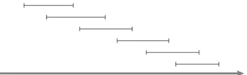
the tree widens very quickly due to the recursive branching. To take a more extreme example, on a nicely layered instance like the one in Figure 6.4, where p(j)=j−2 for eachj=2, 3, 4, . . . ,n, we see thatCompute-Opt(j)generates separate recursive calls on problems of sizesj−1 andj−2. In other words, the total number of calls made to Compute-Opt on this instance will grow
OPT(6)
OPT(5)
OPT(4) OPT(3)
OPT(1)
OPT(2)
OPT(2)
OPT(2) OPT(1)
OPT(1)
OPT(1)
OPT(3)
OPT(1)
OPT(3)
OPT(1)
The tree of subproblems grows very quickly.
Figure 6.3 The tree of subproblems called byCompute-Opton the problem instance of Figure 6.2.
Figure 6.4 An instance of weighted interval scheduling on which the simpleCompute- Optrecursion will take exponential time. The values of all intervals in this instance are 1.
like the Fibonacci numbers, which increase exponentially. Thus we have not achieved a polynomial-time solution.
Memoizing the Recursion
In fact, though, we’re not so far from having a polynomial-time algorithm.
A fundamental observation, which forms the second crucial component of a dynamic programming solution, is that our recursive algorithm Compute- Opt is really only solving n+1 different subproblems: Compute-Opt(0), Compute-Opt(1), . . . ,Compute-Opt(n). The fact that it runs in exponential time as written is simply due to the spectacular redundancy in the number of times it issues each of these calls.
How could we eliminate all this redundancy? We could store the value of Compute-Opt in a globally accessible place the first time we compute it and then simply use this precomputed value in place of all future recursive calls.
This technique of saving values that have already been computed is referred to asmemoization.
We implement the above strategy in the more “intelligent” procedureM- Compute-Opt. This procedure will make use of an arrayM[0 . . .n];M[j] will start with the value “empty,” but will hold the value of Compute-Opt(j) as soon as it is first determined. To determine OPT(n), we invokeM-Compute- Opt(n).
M-Compute-Opt(j) If j=0 then
Return 0
Else if M[j]is not empty then Return M[j]
Else
6.1 Weighted Interval Scheduling: A Recursive Procedure
257
Define M[j] = max(vj+M-Compute-Opt(p(j)), M-Compute-Opt(j−1)) Return M[j]
Endif
Analyzing the Memoized Version
Clearly, this looks very similar to our previous implementation of the algo- rithm; however, memoization has brought the running time way down.
(6.4) The running time ofM-Compute-Opt(n)is O(n)(assuming the input intervals are sorted by their finish times).
Proof. The time spent in a single call toM-Compute-OptisO(1), excluding the time spent in recursive calls it generates. So the running time is bounded by a constant times the number of calls ever issued toM-Compute-Opt. Since the implementation itself gives no explicit upper bound on this number of calls, we try to find a bound by looking for a good measure of “progress.”
The most useful progress measure here is the number of entries inMthat are not “empty.” Initially this number is 0; but each time the procedure invokes the recurrence, issuing two recursive calls toM-Compute-Opt, it fills in a new entry, and hence increases the number of filled-in entries by 1. SinceM has onlyn+1 entries, it follows that there can be at mostO(n)calls toM-Compute- Opt, and hence the running time of M-Compute-Opt(n)isO(n), as desired.
Computing a Solution in Addition to Its Value
So far we have simply computed thevalueof an optimal solution; presumably we want a full optimal set of intervals as well. It would be easy to extend M-Compute-Optso as to keep track of an optimal solution in addition to its value: we could maintain an additional arraySso thatS[i] contains an optimal set of intervals among{1, 2, . . . ,i}. Naively enhancing the code to maintain the solutions in the arrayS, however, would blow up the running time by an additional factor ofO(n): while a position in theM array can be updated in O(1)time, writing down a set in the S array takes O(n)time. We can avoid thisO(n)blow-up by not explicitly maintainingS, but rather by recovering the optimal solution from values saved in the arrayM after the optimum value has been computed.
We know from (6.2) that j belongs to an optimal solution for the set of intervals {1, . . . ,j} if and only if vj+OPT(p(j))≥OPT(j−1). Using this observation, we get the following simple procedure, which “traces back”
through the arrayMto find the set of intervals in an optimal solution.
Find-Solution(j) If j=0 then
Output nothing Else
If vj+M[p(j)]≥M[j−1] then
Output j together with the result of Find-Solution(p(j)) Else
Output the result of Find-Solution(j−1) Endif
Endif
SinceFind-Solutioncalls itself recursively only on strictly smaller val- ues, it makes a total ofO(n)recursive calls; and since it spends constant time per call, we have
(6.5) Given the array M of the optimal values of the sub-problems,Find- Solutionreturns an optimal solution in O(n)time.
6.2 Principles of Dynamic Programming:
Memoization or Iteration over Subproblems
We now use the algorithm for the Weighted Interval Scheduling Problem developed in the previous section to summarize the basic principles of dynamic programming, and also to offer a different perspective that will be fundamental to the rest of the chapter: iterating over subproblems, rather than computing solutions recursively.
In the previous section, we developed a polynomial-time solution to the Weighted Interval Scheduling Problem by first designing an exponential-time recursive algorithm and then converting it (by memoization) to an efficient recursive algorithm that consulted a global array M of optimal solutions to subproblems. To really understand what is going on here, however, it helps to formulate an essentially equivalent version of the algorithm. It is this new formulation that most explicitly captures the essence of the dynamic program- ming technique, and it will serve as a general template for the algorithms we develop in later sections.
Designing the Algorithm
The key to the efficient algorithm is really the arrayM. It encodes the notion that we are using the value of optimal solutions to the subproblems on intervals {1, 2, . . . ,j}for eachj, and it uses (6.1) to define the value ofM[j] based on
6.2 Principles of Dynamic Programming
259
values that come earlier in the array. Once we have the arrayM, the problem is solved:M[n] contains the value of the optimal solution on the full instance, andFind-Solutioncan be used to trace back throughMefficiently and return an optimal solution itself.
The point to realize, then, is that we can directly compute the entries in M by an iterative algorithm, rather than using memoized recursion. We just start withM[0]=0 and keep incrementingj; each time we need to determine a valueM[j], the answer is provided by (6.1). The algorithm looks as follows.
Iterative-Compute-Opt M[0]=0
For j=1, 2, . . . ,n
M[j]=max(vj+M[p(j)],M[j−1]) Endfor
Analyzing the Algorithm
By exact analogy with the proof of (6.3), we can prove by induction onjthat this algorithm writesOPT(j)in array entryM[j]; (6.1) provides the induction step. Also, as before, we can pass the filled-in arrayMtoFind-Solutionto get an optimal solution in addition to the value. Finally, the running time of Iterative-Compute-Opt is clearly O(n), since it explicitly runs for n iterations and spends constant time in each.
An example of the execution ofIterative-Compute-Optis depicted in Figure 6.5. In each iteration, the algorithm fills in one additional entry of the arrayM, by comparing the value ofvj+M[p(j)] to the value ofM[j−1].
A Basic Outline of Dynamic Programming
This, then, provides a second efficient algorithm to solve the Weighted In- terval Scheduling Problem. The two approaches clearly have a great deal of conceptual overlap, since they both grow from the insight contained in the recurrence (6.1). For the remainder of the chapter, we will develop dynamic programming algorithms using the second type of approach—iterative build- ing up of subproblems—because the algorithms are often simpler to express this way. But in each case that we consider, there is an equivalent way to formulate the algorithm as a memoized recursion.
Most crucially, the bulk of our discussion about the particular problem of selecting intervals can be cast more generally as a rough template for designing dynamic programming algorithms. To set about developing an algorithm based on dynamic programming, one needs a collection of subproblems derived from the original problem that satisfies a few basic properties.
Index 1 2 3 4 5 6
p(1) = 0 p(2) = 0 p(3) = 1 p(4) = 0 p(5) = 3 p(6) = 3 w1 = 2
w2 = 4 w3 = 4
w4 = 7 w5 = 2
w6 = 1
2 0
0 1 2 3 4 5 6 M =
2
0 4
2
0 4 6
2
0 4 6 7
2
0 4 6 7 8
2
0 4 6 7 8 8
(a) (b)
Figure 6.5 Part (b) shows the iterations ofIterative-Compute-Opton the sample instance of Weighted Interval Scheduling depicted in part (a).
(i) There are only a polynomial number of subproblems.
(ii) The solution to the original problem can be easily computed from the solutions to the subproblems. (For example, the original problem may actuallybeone of the subproblems.)
(iii) There is a natural ordering on subproblems from “smallest” to “largest,”
together with an easy-to-compute recurrence (as in (6.1) and (6.2)) that allows one to determine the solution to a subproblem from the solutions to some number of smaller subproblems.
Naturally, these are informal guidelines. In particular, the notion of “smaller”
in part (iii) will depend on the type of recurrence one has.
We will see that it is sometimes easier to start the process of designing such an algorithm by formulating a set of subproblems that looks natural, and then figuring out a recurrence that links them together; but often (as happened in the case of weighted interval scheduling), it can be useful to first define a recurrence by reasoning about the structure of an optimal solution, and then determine which subproblems will be necessary to unwind the recurrence.
This chicken-and-egg relationship between subproblems and recurrences is a subtle issue underlying dynamic programming. It’s never clear that a collection of subproblems will be useful until one finds a recurrence linking them together; but it can be difficult to think about recurrences in the absence of the “smaller” subproblems that they build on. In subsequent sections, we will develop further practice in managing this design trade-off.
6.3 Segmented Least Squares: Multi-way Choices
261
6.3 Segmented Least Squares: Multi-way Choices
We now discuss a different type of problem, which illustrates a slightly more complicated style of dynamic programming. In the previous section, we developed a recurrence based on a fundamentallybinary choice: either the interval n belonged to an optimal solution or it didn’t. In the problem we consider here, the recurrence will involve what might be called “multi- way choices”: at each step, we have a polynomial number of possibilities to consider for the structure of the optimal solution. As we’ll see, the dynamic programming approach adapts to this more general situation very naturally.
As a separate issue, the problem developed in this section is also a nice illustration of how a clean algorithmic definition can formalize a notion that initially seems too fuzzy and nonintuitive to work with mathematically.
The Problem
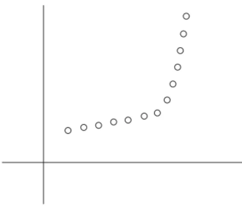
Often when looking at scientific or statistical data, plotted on a two- dimensional set of axes, one tries to pass a “line of best fit” through the data, as in Figure 6.6.
This is a foundational problem in statistics and numerical analysis, formu- lated as follows. Suppose our data consists of a setPofnpoints in the plane, denoted(x1,y1),(x2,y2), . . . ,(xn,yn); and supposex1<x2<. . .<xn. Given a lineLdefined by the equation y=ax+b, we say that theerror ofL with respect toPis the sum of its squared “distances” to the points inP:
Error(L,P)=
n
i=1
(yi−axi−b)2.
Figure 6.6 A “line of best fit.”
Figure 6.7A set of points that lie approximately on two lines.
A natural goal is then to find the line with minimum error; this turns out to have a nice closed-form solution that can be easily derived using calculus.
Skipping the derivation here, we simply state the result: The line of minimum error isy=ax+b, where
a=n
ixiyi−
ixi iyi
n
ix2i −
ixi2 and b=
iyi−a
ixi
n .
Now, here’s a kind of issue that these formulas weren’t designed to cover.
Often we have data that looks something like the picture in Figure 6.7. In this case, we’d like to make a statement like: “The points lie roughly on a sequence of two lines.” How could we formalize this concept?
Essentially, any single line through the points in the figure would have a terrible error; but if we use two lines, we could achieve quite a small error. So we could try formulating a new problem as follows: Rather than seek a single line of best fit, we are allowed to pass an arbitrary set of lines through the points, and we seek a set of lines that minimizes the error. But this fails as a good problem formulation, because it has a trivial solution: if we’re allowed to fit the points with an arbitrarily large set of lines, we could fit the points perfectly by having a different line pass through each pair of consecutive points inP.
At the other extreme, we could try “hard-coding” the number two into the problem; we could seek the best fit using at most two lines. But this too misses a crucial feature of our intuition: We didn’t start out with a preconceived idea that the points lay approximately on two lines; we concluded that from looking at the picture. For example, most people would say that the points in Figure 6.8 lie approximately on three lines.
6.3 Segmented Least Squares: Multi-way Choices
263
Figure 6.8A set of points that lie approximately on three lines.
Thus, intuitively, we need a problem formulation that requires us to fit the points well, using as few lines as possible. We now formulate a problem—
theSegmented Least Squares Problem—that captures these issues quite cleanly.
The problem is a fundamental instance of an issue in data mining and statistics known as change detection: Given a sequence of data points, we want to identify a few points in the sequence at which a discretechange occurs (in this case, a change from one linear approximation to another).
Formulating the Problem As in the discussion above, we are given a set of pointsP= {(x1,y1),(x2,y2), . . . ,(xn,yn)}, withx1<x2<. . .<xn. We will use pi to denote the point (xi,yi). We must first partition P into some number of segments. Eachsegmentis a subset of P that represents a contiguous set ofx-coordinates; that is, it is a subset of the form {pi,pi+1, . . . ,pj−1,pj}for some indicesi≤j. Then, for each segmentSin our partition ofP, we compute the line minimizing the error with respect to the points inS, according to the formulas above.
Thepenaltyof a partition is defined to be a sum of the following terms.
(i) The number of segments into which we partitionP, times a fixed, given multiplierC>0.
(ii) For each segment, the error value of the optimal line through that segment.
Our goal in the Segmented Least Squares Problem is to find a partition of minimum penalty. This minimization captures the trade-offs we discussed earlier. We are allowed to consider partitions into any number of segments; as we increase the number of segments, we reduce the penalty terms in part (ii) of the definition, but we increase the term in part (i). (The multiplierCis provided
with the input, and by tuning C, we can penalize the use of additional lines to a greater or lesser extent.)
There are exponentially many possible partitions ofP, and initially it is not clear that we should be able to find the optimal one efficiently. We now show how to use dynamic programming to find a partition of minimum penalty in time polynomial inn.
Designing the Algorithm
To begin with, we should recall the ingredients we need for a dynamic program- ming algorithm, as outlined at the end of Section 6.2.We want a polynomial number of subproblems, the solutions of which should yield a solution to the original problem; and we should be able to build up solutions to these subprob- lems using a recurrence. As with the Weighted Interval Scheduling Problem, it helps to think about some simple properties of the optimal solution. Note, however, that there is not really a direct analogy to weighted interval sched- uling: there we were looking for asubset ofn objects, whereas here we are seeking topartition nobjects.
For segmented least squares, the following observation is very useful:
The last point pn belongs to a single segment in the optimal partition, and that segment begins at some earlier point pi. This is the type of observation that can suggest the right set of subproblems: if we knew the identity of the last segmentpi, . . . ,pn(see Figure 6.9), then we could remove those points from consideration and recursively solve the problem on the remaining points p1, . . . ,pi−1.
OPT(i – 1) i n
Figure 6.9 A possible solution: a single line segment fits pointspi,pi+1, . . . ,pn,and then an optimal solution is found for the remaining pointsp1,p2, . . . ,pi−1.
6.3 Segmented Least Squares: Multi-way Choices
265
Suppose we let OPT(i) denote the optimum solution for the points p1, . . . ,pi, and we let ei,j denote the minimum error of any line with re- spect topi,pi+1, . . . ,pj. (We will writeOPT(0)=0 as a boundary case.) Then our observation above says the following.
(6.6) If the last segment of the optimal partition is pi, . . . ,pn, then the value of the optimal solution isOPT(n)=ei,n+C+OPT(i−1).
Using the same observation for the subproblem consisting of the points p1, . . . ,pj, we see that to getOPT(j)we should find the best way to produce a final segmentpi, . . . ,pj—paying the error plus an additiveCfor this segment—
together with an optimal solutionOPT(i−1)for the remaining points. In other words, we have justified the following recurrence.
(6.7) For the subproblem on the points p1, . . . ,pj,
OPT(j)=min
1≤i≤j(ei,j+C+OPT(i−1)),
and the segment pi, . . . ,pjis used in an optimum solution for the subproblem if and only if the minimum is obtained using index i.
The hard part in designing the algorithm is now behind us. From here, we simply build up the solutionsOPT(i)in order of increasingi.
Segmented-Least-Squares(n) Array M[0 . . .n]
Set M[0]=0 For all pairs i≤j
Compute the least squares error ei,j for the segment pi, . . . ,pj Endfor
For j=1, 2, . . . ,n
Use the recurrence (6.7) to compute M[j]
Endfor Return M[n]
By analogy with the arguments for weighted interval scheduling, the correctness of this algorithm can be proved directly by induction, with (6.7) providing the induction step.
And as in our algorithm for weighted interval scheduling, we can trace back through the arrayMto compute an optimum partition.
Find-Segments(j) If j=0 then
Output nothing Else
Find an i that minimizes ei,j+C+M[i−1]
Output the segment {pi, . . . ,pj} and the result of Find-Segments(i−1)
Endif
Analyzing the Algorithm
Finally, we consider the running time of Segmented-Least-Squares. First we need to compute the values of all the least-squares errorsei,j. To perform a simple accounting of the running time for this, we note that there areO(n2) pairs (i,j)for which this computation is needed; and for each pair (i,j), we can use the formula given at the beginning of this section to computeei,j in O(n)time. Thus the total running time to compute allei,jvalues isO(n3).
Following this, the algorithm hasniterations, for valuesj=1, . . . ,n. For each value ofj, we have to determine the minimum in the recurrence (6.7) to fill in the array entryM[j]; this takes timeO(n)for eachj, for a total ofO(n2).
Thus the running time isO(n2)once all theei,jvalues have been determined.1
6.4 Subset Sums and Knapsacks: Adding a Variable
We’re seeing more and more that issues in scheduling provide a rich source of practically motivated algorithmic problems. So far we’ve considered problems in which requests are specified by a given interval of time on a resource, as well as problems in which requests have a duration and a deadline but do not mandate a particular interval during which they need to be done.
In this section, we consider a version of the second type of problem, with durations and deadlines, which is difficult to solve directly using the techniques we’ve seen so far. We will use dynamic programming to solve the problem, but with a twist: the “obvious” set of subproblems will turn out not to be enough, and so we end up creating a richer collection of subproblems. As
1In this analysis, the running time is dominated by theO(n3)needed to compute allei,jvalues. But, in fact, it is possible to compute all these values inO(n2)time, which brings the running time of the full algorithm down toO(n2). The idea, whose details we will leave as an exercise for the reader, is to first computeei,jfor all pairs(i,j)wherej−i=1, then for all pairs wherej−i=2, thenj−i=3, and so forth. This way, when we get to a particularei,jvalue, we can use the ingredients of the calculation
forei,j−1to determineei,jin constant time.
6.4 Subset Sums and Knapsacks: Adding a Variable
267
we will see, this is done by adding a new variable to the recurrence underlying the dynamic program.
The Problem
In the scheduling problem we consider here, we have a single machine that can process jobs, and we have a set of requests {1, 2, . . . ,n}. We are only able to use this resource for the period between time 0 and timeW, for some numberW. Each request corresponds to a job that requires timewito process.
If our goal is to process jobs so as to keep the machine as busy as possible up to the “cut-off”W, which jobs should we choose?
More formally, we are given n items {1, . . . ,n}, and each has a given nonnegative weightwi (fori=1, . . . ,n). We are also given a bound W. We would like to select a subsetS of the items so that
i∈Swi≤W and, subject to this restriction,
i∈Swiis as large as possible. We will call this theSubset Sum Problem.
This problem is a natural special case of a more general problem called the Knapsack Problem, where each requestihas both avalue viand aweight wi. The goal in this more general problem is to select a subset of maximum total value, subject to the restriction that its total weight not exceedW. Knapsack problems often show up as subproblems in other, more complex problems. The nameknapsackrefers to the problem of filling a knapsack of capacityW as full as possible (or packing in as much value as possible), using a subset of the items{1, . . . ,n}. We will useweight ortimewhen referring to the quantities wiandW.
Since this resembles other scheduling problems we’ve seen before, it’s natural to ask whether a greedy algorithm can find the optimal solution. It appears that the answer is no—at least, no efficient greedy rule is known that always constructs an optimal solution. One natural greedy approach to try would be to sort the items by decreasing weight—or at least to do this for all items of weight at mostW—and then start selecting items in this order as long as the total weight remains belowW. But ifWis a multiple of 2, and we have three items with weights{W/2+1,W/2,W/2}, then we see that this greedy algorithm will not produce the optimal solution. Alternately, we could sort by increasing weight and then do the same thing; but this fails on inputs like {1,W/2,W/2}.
The goal of this section is to show how to use dynamic programming to solve this problem. Recall the main principles of dynamic programming: We have to come up with a small number of subproblems so that each subproblem can be solved easily from “smaller” subproblems, and the solution to the original problem can be obtained easily once we know the solutions to all
the subproblems. The tricky issue here lies in figuring out a good set of subproblems.
Designing the Algorithm
A False Start One general strategy, which worked for us in the case of Weighted Interval Scheduling, is to consider subproblems involving only the first i requests. We start by trying this strategy here. We use the notation
OPT(i), analogously to the notation used before, to denote the best possible solution using a subset of the requests{1, . . . ,i}. The key to our method for the Weighted Interval Scheduling Problem was to concentrate on an optimal solutionOto our problem and consider two cases, depending on whether or not the last request nis accepted or rejected by this optimum solution. Just as in that case, we have the first part, which follows immediately from the definition ofOPT(i).
. Ifn∈O, thenOPT(n)=OPT(n−1).
Next we have to consider the case in whichn∈O. What we’d like here is a simple recursion, which tells us the best possible value we can get for solutions that contain the last request n. For Weighted Interval Scheduling this was easy, as we could simply delete each request that conflicted with request n. In the current problem, this is not so simple. Accepting requestn does not immediately imply that we have to reject any other request. Instead, it means that for the subset of requestsS⊆ {1, . . . ,n−1}that we will accept, we have less available weight left: a weight of wn is used on the accepted request n, and we only have W−wn weight left for the setS of remaining requests that we accept. See Figure 6.10.
A Better Solution This suggests that we need more subproblems: To find out the value forOPT(n)we not only need the value ofOPT(n−1), but we also need to know the best solution we can get using a subset of the first n−1 items and total allowed weight W−wn. We are therefore going to use many more subproblems: one for each initial set{1, . . . ,i}of the items, and each possible
W
wn
Figure 6.10 After itemnis included in the solution, a weight ofwnis used up and there isW−wnavailable weight left.
6.4 Subset Sums and Knapsacks: Adding a Variable
269
value for the remaining available weightw. Assume thatW is an integer, and all requestsi=1, . . . ,nhave integer weightswi. We will have a subproblem for eachi=0, 1, . . . ,nand each integer 0≤w≤W. We will useOPT(i,w)to denote the value of the optimal solution using a subset of the items{1, . . . ,i}
with maximum allowed weightw, that is,
OPT(i,w)=max
S
j∈S
wj,
where the maximum is over subsetsS⊆ {1, . . . ,i}that satisfy
j∈Swj≤w.
Using this new set of subproblems, we will be able to express the value
OPT(i,w) as a simple expression in terms of values from smaller problems.
Moreover,OPT(n,W)is the quantity we’re looking for in the end. As before, letOdenote an optimum solution for the original problem.
. If n∈O, then OPT(n,W)=OPT(n−1,W), since we can simply ignore itemn.
. Ifn∈O, thenOPT(n,W)=wn+OPT(n−1,W−wn), since we now seek to use the remaining capacity ofW−wnin an optimal way across items 1, 2, . . . ,n−1.
When thenthitem is too big, that is,W<wn, then we must haveOPT(n,W)=
OPT(n−1,W). Otherwise, we get the optimum solution allowing allnrequests by taking the better of these two options. Using the same line of argument for the subproblem for items{1, . . . ,i}, and maximum allowed weightw, gives us the following recurrence.
(6.8) If w<wi thenOPT(i,w)=OPT(i−1,w). Otherwise
OPT(i,w)=max(OPT(i−1,w),wi+OPT(i−1,w−wi)).
As before, we want to design an algorithm that builds up a table of all
OPT(i,w)values while computing each of them at most once.
Subset-Sum(n,W) Array M[0 . . .n, 0 . . .W]
Initialize M[0,w]=0 for each w=0, 1, . . . ,W For i=1, 2, . . . ,n
For w=0, . . . ,W
Use the recurrence (6.8) to compute M[i,w]
Endfor Endfor
Return M[n,W]
0 0 0 0 0 0 0 0 0 0 0
0 0 0 0 0 0 0 0 0 0 0 0 0 0 0 n
i i – 1
2 1 0
0 1 2 w–wi w W
Figure 6.11 The two-dimensional table ofOPTvalues. The leftmost column and bottom row is always 0. The entry for OPT(i,w) is computed from the two other entries OPT(i−1,w)andOPT(i−1,w−wi), as indicated by the arrows.
Using (6.8) one can immediately prove by induction that the returned value M[n,W] is the optimum solution value for the requests 1, . . . ,nand available weightW.
Analyzing the Algorithm
Recall the tabular picture we considered in Figure 6.5, associated with weighted interval scheduling, where we also showed the way in which the ar- ray M for that algorithm was iteratively filled in. For the algorithm we’ve just designed, we can use a similar representation, but we need a two- dimensional table, reflecting the two-dimensional array of subproblems that is being built up. Figure 6.11 shows the building up of subproblems in this case: the valueM[i,w] is computed from the two other valuesM[i−1,w] and M[i−1,w−wi].
As an example of this algorithm executing, consider an instance with weight limitW=6, andn=3 items of sizesw1=w2=2 andw3=3. We find that the optimal valueOPT(3, 6)=5 (which we get by using the third item and one of the first two items). Figure 6.12 illustrates the way the algorithm fills in the two-dimensional table ofOPTvalues row by row.
Next we will worry about the running time of this algorithm. As before in the case of weighted interval scheduling, we are building up a table of solutions M, and we compute each of the valuesM[i,w] inO(1)time using the previous values. Thus the running time is proportional to the number of entries in the table.
6.4 Subset Sums and Knapsacks: Adding a Variable
271
0
0 0 0 0 0 0
0 1 2 3 Initial values
4 5 6 3
2 1
0 0 0 0 0 0 0 0
0
0 2 2 2 2 2
0 1 2 3
Filling in values for i = 1 4 5 6 3
2 1 0
0
0 0 0 0 0 0
0
0 2 2 2 2 2 0 0 2 2 2 2 2
0
0 2 3 4 5 5
0
0 2 2 4 4 4 0 0 2 2 4 4 4
0 1 2 3
Filling in values for i = 2 4 5 6 3
2 1
0 0 0 0 0 0 0 0
0 1 2 3
Filling in values for i = 3 4 5 6 3
2 1 0
Knapsack size W = 6, items w1 = 2, w2 = 2, w3 = 3
Figure 6.12 The iterations of the algorithm on a sample instance of the Subset Sum Problem.
(6.9) The Subset-Sum(n,W) Algorithm correctly computes the optimal value of the problem, and runs in O(nW)time.
Note that this method is not as efficient as our dynamic program for the Weighted Interval Scheduling Problem. Indeed, its running time is not a polynomial function ofn; rather, it is a polynomial function of nand W, the largest integer involved in defining the problem. We call such algorithms pseudo-polynomial. Pseudo-polynomial algorithms can be reasonably efficient when the numbers{wi}involved in the input are reasonably small; however, they become less practical as these numbers grow large.
To recover an optimal setSof items, we can trace back through the array Mby a procedure similar to those we developed in the previous sections.
(6.10) Given a table M of the optimal values of the subproblems, the optimal set S can be found in O(n)time.
Extension: The Knapsack Problem
The Knapsack Problem is a bit more complex than the scheduling problem we discussed earlier. Consider a situation in which each itemihas a nonnegative weightwi as before, and also a distinctvalue vi. Our goal is now to find a
subset S of maximum value
i∈Svi, subject to the restriction that the total weight of the set should not exceedW:
i∈Swi≤W.
It is not hard to extend our dynamic programming algorithm to this more general problem. We use the analogous set of subproblems,OPT(i,w), to denote the value of the optimal solution using a subset of the items {1, . . . ,i}and maximum available weightw. We consider an optimal solutionO, and identify two cases depending on whether or notn∈O.
. Ifn∈O, thenOPT(n,W)=OPT(n−1,W).
. Ifn∈O, thenOPT(n,W)=vn+OPT(n−1,W−wn).
Using this line of argument for the subproblems implies the following analogue of (6.8).
(6.11) If w<wi thenOPT(i,w)=OPT(i−1,w). Otherwise
OPT(i,w)=max(OPT(i−1,w),vi+OPT(i−1,w−wi)).
Using this recurrence, we can write down a completely analogous dynamic programming algorithm, and this implies the following fact.
(6.12) The Knapsack Problem can be solved in O(nW)time.
6.5 RNA Secondary Structure: Dynamic Programming over Intervals
In the Knapsack Problem, we were able to formulate a dynamic programming algorithm by adding a new variable. A different but very common way by which one ends up adding a variable to a dynamic program is through the following scenario. We start by thinking about the set of subproblems on {1, 2, . . . ,j}, for all choices of j, and find ourselves unable to come up with a natural recurrence. We then look at the larger set of subproblems on {i,i+1, . . . ,j} for all choices of i and j (where i≤j), and find a natural recurrence relation on these subproblems. In this way, we have added the second variablei; the effect is to consider a subproblem for every contiguous interval in{1, 2, . . . ,n}.
There are a few canonical problems that fit this profile; those of you who have studied parsing algorithms for context-free grammars have probably seen at least one dynamic programming algorithm in this style. Here we focus on the problem of RNA secondary structure prediction, a fundamental issue in computational biology.
6.5 RNA Secondary Structure: Dynamic Programming over Intervals
273
U A
C G
G C
A
G C
A G
C
A U
G
G A C
C U G C A C U
A G
G
C A G
U A U U
A G
G A C U
A
G C
A A
Figure 6.13An RNA secondary structure. Thick lines connect adjacent elements of the sequence; thin lines indicate pairs of elements that are matched.
The Problem
As one learns in introductory biology classes, Watson and Crick posited that double-stranded DNA is “zipped” together by complementary base-pairing.
Each strand of DNA can be viewed as a string ofbases, where each base is drawn from the set{A,C,G,T}.2The basesAandTpair with each other, and the basesCandGpair with each other; it is theseA-T andC-Gpairings that hold the two strands together.
Now, single-stranded RNA molecules are key components in many of the processes that go on inside a cell, and they follow more or less the same structural principles. However, unlike double-stranded DNA, there’s no
“second strand” for the RNA to stick to; so it tends to loop back and form base pairs with itself, resulting in interesting shapes like the one depicted in Figure 6.13. The set of pairs (and resulting shape) formed by the RNA molecule through this process is called the secondary structure, and understanding the secondary structure is essential for understanding the behavior of the molecule.
2Adenine, cytosine, guanine, and thymine, the four basic units of DNA.
For our purposes, a single-stranded RNA molecule can be viewed as a sequence ofnsymbols (bases) drawn from the alphabet{A,C,G,U}.3LetB= b1b2. . .bnbe a single-stranded RNA molecule, where eachbi∈ {A,C,G,U}.
To a first approximation, one can model its secondary structure as follows. As usual, we require thatA pairs with U, andC pairs with G; we also require that each base can pair with at most one other base—in other words, the set of base pairs forms amatching. It also turns out that secondary structures are (again, to a first approximation) “knot-free,” which we will formalize as a kind ofnoncrossing condition below.
Thus, concretely, we say that asecondary structure on Bis a set of pairs S= {(i,j)}, wherei,j∈ {1, 2, . . . ,n}, that satisfies the following conditions.
(i) (No sharp turns.)The ends of each pair inSare separated by at least four intervening bases; that is, if(i,j)∈S, theni<j−4.
(ii) The elements of any pair inSconsist of either{A,U}or{C,G}(in either order).
(iii) Sis a matching: no base appears in more than one pair.
(iv) (The noncrossing condition.)If(i,j)and(k,ℓ)are two pairs inS, then we cannot havei<k<j< ℓ. (See Figure 6.14 for an illustration.) Note that the RNA secondary structure in Figure 6.13 satisfies properties (i) through (iv). From a structural point of view, condition (i) arises simply because the RNA molecule cannot bend too sharply; and conditions (ii) and (iii) are the fundamental Watson-Crick rules of base-pairing. Condition (iv) is the striking one, since it’s not obvious why it should hold in nature. But while there are sporadic exceptions to it in real molecules (via so-called pseudo- knotting), it does turn out to be a good approximation to the spatial constraints on real RNA secondary structures.
Now, out of all the secondary structures that are possible for a single RNA molecule, which are the ones that are likely to arise under physiological conditions? The usual hypothesis is that a single-stranded RNA molecule will form the secondary structure with the optimum total free energy. The correct model for the free energy of a secondary structure is a subject of much debate;
but a first approximation here is to assume that the free energy of a secondary structure is proportional simply to thenumberof base pairs that it contains.
Thus, having said all this, we can state the basic RNA secondary structure prediction problem very simply: We want an efficient algorithm that takes
3Note that the symbolTfrom the alphabet of DNA has been replaced by aU, but this is not important for us here.
6.5 RNA Secondary Structure: Dynamic Programming over Intervals
275
C
C A
G G
(a) (b)
A U G U
A C A U G A U G G C C A U G U U
G U A C A
Figure 6.14 Two views of an RNA secondary structure. In the second view, (b), the string has been “stretched” lengthwise, and edges connecting matched pairs appear as noncrossing “bubbles” over the string.
a single-stranded RNA moleculeB=b1b2. . .bnand determines a secondary structureSwith the maximum possible number of base pairs.
Designing and Analyzing the Algorithm
A First Attempt at Dynamic Programming The natural first attempt to apply dynamic programming would presumably be based on the following subproblems: We say thatOPT(j)is the maximum number of base pairs in a secondary structure onb1b2. . .bj. By the no-sharp-turns condition above, we know thatOPT(j)=0 forj≤5; and we know thatOPT(n)is the solution we’re looking for.
The trouble comes when we try writing down a recurrence that expresses
OPT(j)in terms of the solutions to smaller subproblems. We can get partway there: in the optimal secondary structure onb1b2. . .bj, it’s the case that either
. jis not involved in a pair; or
. jpairs withtfor somet<j−4.
In the first case, we just need to consult our solution forOPT(j−1). The second case is depicted in Figure 6.15(a); because of the noncrossing condition, we now know that no pair can have one end between 1 and t−1 and the other end between t+1 and j−1. We’ve therefore effectively isolated two new subproblems: one on the basesb1b2. . .bt−1, and the other on the bases bt+1. . .bj−1. The first is solved byOPT(t−1), but the second is not on our list of subproblems, because it does not begin withb1.
(a)
1 2 t – 1 t t + 1 j – 1 j
(b)
i t – 1 t t + 1 j – 1 j
Including the pair (t,j) results in two independent subproblems.
Figure 6.15 Schematic views of the dynamic programming recurrence using (a) one variable, and (b) two variables.
This is the insight that makes us realize we need to add a variable. We need to be able to work with subproblems that do not begin withb1; in other words, we need to consider subproblems onbibi+1. . .bjfor all choices ofi≤j.
Dynamic Programming over Intervals Once we make this decision, our previous reasoning leads straight to a successful recurrence. LetOPT(i,j)denote the maximum number of base pairs in a secondary structure onbibi+1. . .bj. The no-sharp-turns condition lets us initializeOPT(i,j)=0 wheneveri≥j−4.
(For notational convenience, we will also allow ourselves to refer toO