Chapter 5—Predicted A-X Transition Frequencies and 2-Dimensional Torsion-Torsion Potential Energy Surfaces of HOCH

Chapter 5—Predicted A-X Transition Frequencies and 2-Dimensional Torsion-Torsion Potential Energy Surfaces of HOCH

2

OO• and HOC(CH

3

)

2

OO•

Abstract

In Chapter 4, we presented the 1 (OH stretch) vibrational and A-X electronic spectra of the hydroxymethylperoxy radical (HOCH2OO•, or HMP). The slight red shift in the 1 absorption band suggests the formation of a weak intramolecular hydrogen bond, possibly leading to coupling of vibrational modes (similar to our observations of HOONO in Chapter 3). We observed four clear peaks in the A-X spectrum, consistent with assignment as the hot bands and combination bands with the OOCO torsional mode.

We would like to make the most accurate assignment of the A-X spectrum and assessment of the torsional mode coupling. Although quantum chemistry methods for determining spectroscopic properties of alkyl peroxy radicals have been developed, these methods may or may not be applicable to substituted peroxy systems such as HMP.

In this thesis chapter, we predict the A-X electronic transition frequency and the extent of torsional mode coupling through quantum chemistry methods. We calculate potential energy surfaces as a function of the two torsional modes of HMP (OCOH, OOCO) for both the X and A states at a variety of levels of theory and bases. We also use composite methods to determine the A-X transition frequency. We also extend our methods to the product of HO2 + acetone, HOC(CH3)2OO• (2-hydroxyisopropylperoxy, 2-HIPP) to provide predictions of spectroscopic bands for future studies. Our potential energy surfaces indicate that further studies must be carried out to determine the best overall method for calculation of the spectroscopic properties of substituted alkyl peroxies such as HMP.

Introduction

In Chapter 4, we presented the mid-IR and near-IR spectra of the products of the HO2 + HCHO reaction. Based on our chemistry analysis, kinetics modeling, band simulations, and preliminary quantum chemistry calculations, we assigned both spectra to the primary product HOCH2OO• (HMP, Reaction 5.1): the mid-IR spectrum to the 1

(OH stretch) vibrational mode, and the near-IR spectrum to the A-X electronic transitions.

(5.1) At the end of Chapter 4, we made two key observations about each spectrum when comparing to the spectra of similar molecules. First, the position of the 1 band of HMP (3622 cm⁻¹) is red shifted from the 1 bands of methanol (3681 cm⁻¹) and ethanol (3675 cm⁻¹).⁴⁰ We have already observed (HOONO, Chapter 3) that the formation of internal hydrogen bonds can cause red shifts in the OH stretch frequency. In HMP, interaction between the peroxy (OO) and hydroxy (OH) groups will cause this red shift.

The bond is likely weaker than in HOONO due to the magnitude of the red shifts (60 cm⁻¹ in HMP, 270 cm⁻¹ in HOONO). Nonetheless, even a weak interaction may cause coupling between vibrational modes involving the peroxy and hydroxy groups, notably the two torsions OOCO (15) and HOCO (13), causing extra complexity in the vibrational spectrum.

Second, we observed some qualitative differences between the A-X spectrum of HMP and CH3OO•.¹²² In the HMP spectrum, we observe the OOCO torsional combination band 15¹₀, but do not observe the sequence band 15¹₁. The opposite holds true

in CH3OO•: Chung et al. observe the methyl torsion sequence band 12¹₁, but not the combination band 12¹₀. Given this discrepancy, it is important to confirm the assignment of our HMP spectrum. The possible torsional coupling suggested by the 1 spectrum makes this task harder, as all of the assigned bands could be affected by HMP’s internal hydrogen bond.

Within the last 15 years, Terry Miller and co-workers have developed a general framework for modeling the electronic transitions of alkylperoxy radicals.⁴⁴ Miller uses G2,¹²³ a composite quantum chemistry method (explained in Appendix C) to obtain X and A state energies of alkylperoxies. The accuracy of these calculations is 10–200 cm⁻¹. Predictions are most accurate for small molecules (such as CH3OO•), and get worse with increasing size (such as 3-pentylperoxy)⁴⁴ or halogenation of the alkyl chain (such as CF3OO•).¹²⁴ Both molecules above can be thought of as substituted versions of methylperoxy (3-pentylperoxy replacing two of the H on CH3OO• with C2H5, CF3OO•

simply replacing all hydrogens with fluorines). Substitution may affect the electronic structure and interactions of the peroxy group with the rest of the radical. Thus, there is no guarantee that the G2 method commonly employed for prediction of peroxy spectra will be adequate for HMP, a substituted alkylperoxy with internal hydrogen bonding involving the peroxy group.

The “holy grail” of the spectroscopic studies presented in Chapter 4 is to detect the primary product of HO2 + acetone (Reaction 5.2): HOC(CH3)2OO•

(2-hydroxyisopropylperoxy, or 2-HIPP).

(5.2) Recent studies have shown that HO2 disappears faster in the presence of acetone;

however, by monitoring HO2 alone, these studies cannot differentiate between Reaction 5.2 and an enhancement of HO2 self-reaction. Direct spectroscopic detection of 2-HIPP would provide evidence that Reaction 5.2 does in fact take place. However, there are no predictions as to where the spectroscopic bands of 2-HIPP should be located. In order to make a meaningful prediction of the 2-HIPP spectrum, we must first determine an appropriate method for modeling 2-HIPP.

In this thesis chapter, we present two dimensional potential energy surfaces for the ground (X) and first excited (A) states of HMP, as a function of the OCOH and OOCO dihedral angles. These surfaces were analyzed to determine the extent of torsion- torsion coupling due to internal hydrogen bonding. We also determine the A-X transition frequency on the basis of these calculations. By carrying these calculations out at a wide variety of levels of theory and bases, we can determine appropriate methods for modeling substituted alkyl peroxies such as HMP. We then extend our results to predict the 1 and A-X spectra of 2-HIPP.

Methods

All quantum chemistry calculations in this chapter were performed in Gaussian 03W.⁷⁹ We used three single processor, single core, Windows XP PCs (Caltech).

Potential energy surface data were compiled in GaussView 3.09,¹²⁵ and the resulting plots were generated in SigmaPlot 8.0.¹²⁶

We generated potential energy surfaces of HMP as a function of the two dihedral angles OCOH and OOCO by performing relaxed energy scans (i.e., for each set of dihedral angles (OCOH, OOCO), all other molecular coordinates were allowed to relax).

A-X transition frequencies were obtained by performing a geometry optimization in both the A and X states, then subtracting the difference in energies. This transition frequency was scaled to HO2 (Equation 5.3) to correct for systematic errors in the quantum chemistry method and zero point energy effects.

     



²2



A-X,HO actual A-X,HMP actual A-X,HMP calc

A-X,HO calc

E E E

  E (5.3),

where (EA-X,HO2)actual = 7029 cm⁻¹.⁵⁴

Based on the results of these potential energy surfaces, we examined the global minimum of the X state and the associated potential energy well of the A state in greater detail to obtain information about the A-X transition frequency. We calculated the geometries, energies, and vibrational frequencies of the wells in the X and A states, making use of anharmonic frequency calculations (VPT2) when available in Gaussian 03W. The resulting energy differences were scaled to HO2 according to Equation 5.3 in order to make the best estimates of the A-X transition frequency.

Geometries and energies for the excited (A) state of HMP were obtained by

“freezing” the electrons in the excited state configuration at each step of the self- consistent field calculation, similar to the method developed by Miller and co-workers (see Appendix C for details of this method).⁴⁴

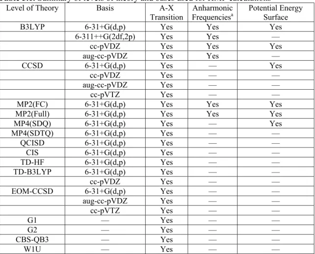
The specific levels of theory and bases used for this study are summarized in Table 5.1. Note that in Gaussian 03W and 09W, anharmonic frequencies are only available at the HF, B3LYP, and MP2 levels of theory.

Table 5.1. Summary of levels of theory and bases used for HMP calculations Level of Theory Basis A-X

Transition

Anharmonic Frequencies^a

Potential Energy Surface B3LYP 6-31+G(d,p) Yes Yes Yes

6-311++G(2df,2p) Yes Yes — cc-pVDZ Yes Yes Yes aug-cc-pVDZ Yes Yes — CCSD 6-31+G(d,p) Yes — Yes

cc-pVDZ Yes — —

aug-cc-pVDZ Yes — —

cc-pVTZ Yes — —

MP2(FC) 6-31+G(d,p) Yes Yes Yes MP2(Full) 6-31+G(d,p) Yes Yes Yes MP4(SDQ) 6-31+G(d,p) Yes — Yes MP4(SDTQ) 6-31+G(d,p) Yes — —

QCISD 6-31+G(d,p) Yes — — CIS 6-31+G(d,p) Yes — — TD-HF 6-31+G(d,p) Yes — — TD-B3LYP 6-31+G(d,p) Yes — —

cc-pVDZ Yes — —

EOM-CCSD 6-31+G(d,p) Yes — — aug-cc-pVDZ Yes — —

cc-pVTZ Yes — —

G1 — Yes — —

G2 — Yes — —

CBS-QB3 — Yes — —

W1U — Yes — —

a) Anharmonic frequencies not available in Gaussian 03W for CCSD, MP4, QCISD, or composite methods

Results

We present the results of our study in three parts. First, we present the 2-dimensional torsional potential energy surfaces of HMP. We show the molecular geometries of the local minima in both the X and A states. The potential energy surfaces show evidence of torsional mode coupling in the X state, but not the A state. These surfaces show that density functional theory and coupled cluster methods are able to

locate all three conformers of HMP on the X state, but Möller-Plesset perturbation theory is not able to locate one of the conformers. Second, we present the vibrational and A-X transition frequencies calculated using density functional, coupled cluster, perturbation, equation of motion, and composite quantum chemistry methods. We observe generally good agreement between experiment and theory across most of these methods. We conclude that density functional, coupled cluster, and composite methods based on these levels of theory are appropriate for modeling HMP. Third, we extend our study to 2-HIPP, predicting the vibrational and A-X bands. We predict 2-HIPP to have an A-X frequency in the range 7900–8000 cm⁻¹, significantly to the blue of HMP.

Torsion-Torsion Potential Energy Surfaces of HMP

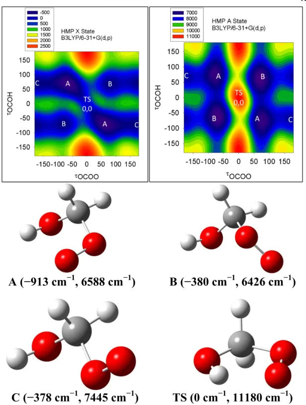
Figures 5.1–5.3 show a series of 2-dimensional potential energy surfaces of HMP as a function of the two dihedral angles OCOH and OOCO. Figure 5.1 shows the B3LYP/6-31+G(d,p) calculated X and A surfaces with the three minima and (OCOH, OOCO)=(0°, 0°) transition state (TS) labeled. Figure 5.2 shows the X and A state potential energy surfaces for the remaining DFT and coupled-cluster calculations:

B3LYP/cc-pVDZ and CCSD/6-31+G(d,p). Figure 5.3 shows the surfaces from the three perturbation theory calculations: MP2(FC)/6-31+G(d,p), MP2(Full)/6-31+(d,p), and MP4(SDQ)/6-31+G(d,p).

A (−913 cm

⁻¹

, 6588 cm

⁻¹

) B (−380 cm

⁻¹

, 6426 cm

⁻¹

)

C (−378 cm

⁻¹

, 7445 cm

⁻¹

)

TS (0 cm

⁻¹

, 11180 cm

⁻¹

)

Figure 5.1. B3LYP/6-31+G(d,p) potential energy surfaces of HMP for the X state (left) and A state (right), as a function of the dihedral angles OCOH and OOCO. The local minima (A, B, C) at the X state geometries, and Cs transition state (TS), are labeled on each surface. The listed energies (X state, A state) are relative to the X state of TS, unscaled. The geometries of these conformers are shown below the surfaces. Energies on the potential energy surfaces are in cm⁻¹, relative to the X state Cs transition state energy.

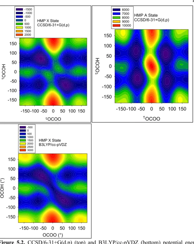
Figure 5.2. CCSD/6-31+G(d,p) (top) and B3LYP/cc-pVDZ (bottom) potential energy surfaces of HMP for the X state (left) and A state (right), as a function of the dihedral angles OCOH and OOCO. Energies on the potential energy surfaces are in cm⁻¹, relative to the X state Cs transition state energy.

HMP X State CCSD/6-31+G(d,p)

OCOO

-150-100 -50 0 50 100 150

OCOH

-150 -100 -50 0 50 100 150

-1500 -1000 -500 0 500 1000 1500 2000

HMP A State CCSD/6-31+G(d,p)

OCOO

-150-100 -50 0 50 100 150

OCOH

-150 -100 -50 0 50 100 150

6000 7000 8000 9000 10000

HMP X State B3LYP/cc-pVDZ

OCOO (°)

-150-100 -50 0 50 100 150

OCOH (°)

-150 -100 -50 0 50 100 150

-500 0 500 1000 1500 2000 2500 3000

HMP X State MP2(FC)/6-31+G(d,p)

OCOO

-150-100 -50 0 50 100 150

OCOH

-150 -100 -50 0 50 100 150

-1000 -500 0 500 1000 1500 2000 2500

HMP A State

MP2(FC)/6-31+G(d,p)

OCOO

-150-100 -50 0 50 100 150

OCOH

-150 -100 -50 0 50 100 150

6000 7000 8000 9000 10000

HMP X State

MP2(Full)/6-31+G(d,p)

OCOO

-150-100 -50 0 50 100 150

OCOH

-150 -100 -50 0 50 100 150

-1000 -500 0 500 1000 1500 2000 2500

HMP A State

MP2(Full)/6-31+G(d,p)

OCOO

-150-100 -50 0 50 100 150

OCOH

-150 -100 -50 0 50 100 150

6000 7000 8000 9000 10000

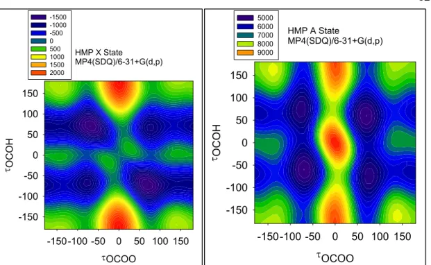
Figure 5.3. MP2(FC)/6-31+G(d,p) (top of previous page), MP2(Full)/6-31+(d,p) (bottom of previous page), and MP4(SDQ)/6-31+G(d,p) (this page) potential energy surfaces of HMP for the X state (left) and A state (right), as a function of the dihedral angles OCOH

and OOCO. Energies on the potential energy surfaces are in cm^-1, relative to the X state Cs

transition state energy.

First, consider the X state surface and energies presented in Figure 5.1 (B3LYP/6-31+G(d,p)). There are three nonequivalent minima on the potential energy surface representing rotation of the peroxy group, similar to the three equivalent minima observed for CH3OO•.¹²⁷ The global minimum conformer (Figure 5.1, labeled Conformer A) features an internal hydrogen bond. At B3LYP/6-31G(d,p), the energy stabilization provided by this hydrogen bond is 550 cm⁻¹, calculated by comparison to the two nonhydrogen bound conformers (B and C). The potential energy well is off axis (diagonal on the OCOH, OCOO plot), indicating that the two torsional modes are coupled to each other.

HMP X State

MP4(SDQ)/6-31+G(d,p)

OCOO

-150-100 -50 0 50 100 150

OCOH

-150 -100 -50 0 50 100 150

-1500 -1000 -500 0 500 1000 1500 2000

HMP A State

MP4(SDQ)/6-31+G(d,p)

OCOO

-150-100 -50 0 50 100 150

OCOH

-150 -100 -50 0 50 100 150

5000 6000 7000 8000 9000

The TS is not a maximum on the surface; at least 1000 cm⁻¹ is required to move from TS to B. Rather, it is a saddle point, and any HMP in the TS conformer will convert to conformer A without any energy barrier. Although the TS appears to have an internal hydrogen bond, it is actually higher in energy than the three minima, likely due to unfavorable orbital overlap from placing the OH and OO groups’ relative orientation.

Clearly there is interaction between these two groups in TS: the minimum energy path is also off axis.

Next consider the A state surface and energies in Figure 5.1. There are still three minima, but there are several qualitative differences compared to the X state surface.

First, we observe that all three minima are on-axis, and the energy of Conformer A is approximately equal to Conformer B (in fact, Conformer B is now the global minimum by 150 cm⁻¹). These two facts imply that there is no hydrogen bonding in the A state of HMP. Second, TS is now a maximum on the surface rather than a saddle point. This affords the possibility of TS being converted into either Conformer A or B. Finally, we note that the positions of the minima on the X state (the positions of the letters) do not match exactly with the minima on the A state. In particular, the wells for conformer A are slightly shifted in OOCO.

The potential energy surfaces in Figure 5.2, when compared to Figure 5.1, show the effects of increasing the level of theory (from B3LYP to CCSD) while keeping the basis set constant (6-31+G(d,p)), and changing the basis set (from 6-31+G(d,p) to cc-pVDZ) while keeping the level of theory constant (B3LYP). The CCSD/6-31+G(d,p) surfaces have the same qualitative features as the B3LYP/6-31+G(d,p) surfaces. On the X state surface, we still observe three local minima with one hydrogen bonded conformer

(normal modes coupled) stabilized by 550 cm⁻¹ compared to the other two conformers.

The A state still shows three minima, none with normal mode coupling, and Conformer B is slightly lower in energy than Conformer A (−200 cm⁻¹). The main difference between the CCSD/6-31+G(d,p) and B3LYP/6-31+G(d,p) surfaces is the relative energy of TS (900 cm⁻¹ above conformer A at B3LYP, 1700 cm⁻¹ at CCSD). Nonetheless, the qualitative agreement between the B3LYP and CCSD surfaces suggests that B3LYP may be a good method for modeling our HO2 + carbonyl systems.

Comparison of the B3LYP/cc-pVDZ surface to the B3LYP/6-31+G(d,p) surface reveals some similarities (three minima, one hydrogen bound) and some significant qualitative changes: widening of the TS saddle point and reduced barrier heights between conformers. This is likely due to the relative inflexibility of the cc-pVDZ basis set (no polarization or diffuse functions) compared to the 6-31+G(d,p) basis. Similar surfaces at aug-cc-pVDZ (not shown here) did agree qualitatively with the 6-31+G(d,p) surface, indicating that polarization and diffuse functions are required to model the HMP radical properly.

Finally, there is one disturbing difference between the perturbation method surfaces (Figure 5.3) and the B3LYP/CCSD surfaces (Figures 5.1 and 5.2). The barrier between Conformers C and A was 75 cm⁻¹ (B3LYP/6-31+G(d,p)) or 100 cm⁻¹ (CCSD/6-31+G(d,p)), and we can therefore calculate properties of conformer C at these two levels of theory. In contrast, at MP2(FC), MP2(Full), or MP4(SDQ), Conformer C is no longer a minimum; rather, it is a shelf (similar to the cis-perp region of HOONO from Chapter 3).

Calculated A-X Transition Frequencies

The most important conformers of HMP in our experiments will be conformers A and B. These potential energy wells are relatively deep (Figures 5.1–5.3); a radical in these conformations will be bound by >900 cm⁻¹ (conformer A) or 280 cm⁻¹ (conformer B), as calculated at B3LYP/6-31+G(d,p). We therefore focus our attention on calculating the A-X transition frequencies out of these two conformations, with the global minimum (conformer A) being the most important due to its very deep well depth.

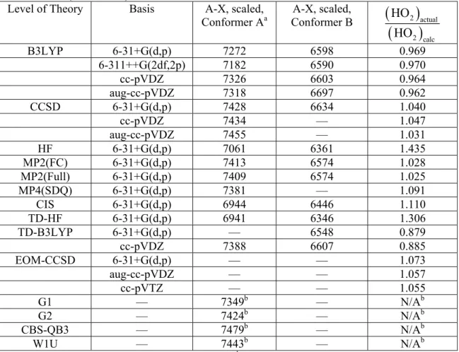
Tables 5.2–5.5 summarize the calculated A-X frequencies, OOCO torsion frequencies in the A and X states, and OH stretch frequencies. In Table 5.2, we scale all of the transition frequencies to HO2 using Equation 5.3. In Tables 5.3-5.5, we calculate anharmonic frequencies using two methods: scaling the harmonic frequencies using known scaling factors,¹²⁸ or directly calculating anharmonic frequencies in Gaussian 09.¹²¹ In Figures 5.4–5.7, we show the deviations of each method’s calculated frequencies to the experimentally determined values (Chapter 4). We discuss the data in these tables and figures after Figure 5.7.

Table 5.2. Calculated A-X transition frequencies (cm⁻¹) of HMP conformers A and B, scaled to HO2 (7029 cm⁻¹).⁵⁴

Level of Theory Basis A-X, scaled, Conformer A^a

A-X, scaled,

Conformer B

 



^{2 actual}_{2 calc}



HO HO

B3LYP 6-31+G(d,p) 7272 6598 0.969 6-311++G(2df,2p) 7182 6590 0.970 cc-pVDZ 7326 6603 0.964 aug-cc-pVDZ 7318 6697 0.962 CCSD 6-31+G(d,p) 7428 6634 1.040

cc-pVDZ 7434 — 1.047 aug-cc-pVDZ 7455 — 1.031

HF 6-31+G(d,p) 7061 6361 1.435 MP2(FC) 6-31+G(d,p) 7413 6574 1.028 MP2(Full) 6-31+G(d,p) 7409 6574 1.025 MP4(SDQ) 6-31+G(d,p) 7381 — 1.091

CIS 6-31+G(d,p) 6944 6446 1.110 TD-HF 6-31+G(d,p) 6941 6346 1.306 TD-B3LYP 6-31+G(d,p) — 6548 0.879

cc-pVDZ 7388 6607 0.885 EOM-CCSD 6-31+G(d,p) — — 1.073

aug-cc-pVDZ — — 1.057 cc-pVTZ — — 1.055

G1 — 7349^b — N/A^b

G2 — 7424^b — N/A^b

CBS-QB3 — 7479^b — N/A^b W1U — 7443^b — N/A^b a) Observed A-X frequency of Conformer A is 7391 cm⁻¹ (Chapter 4)

b) Composite methods are not scaled to HO2

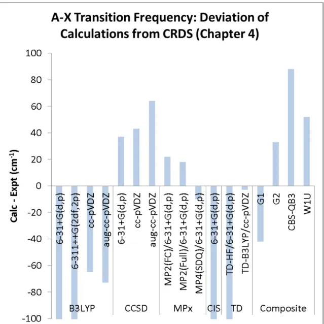
Figure 5.4. Deviation of calculated A-X frequency of HMP from experiment (CRDS, Chapter 4).

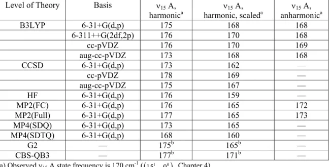
Table 5.3. Calculated 15 (OOCO torsion) frequency for the A state of HMP conformer A, harmonic, harmonic scaled,¹²⁸ and anharmonic.

Level of Theory Basis ₁₅ A, harmonic^a

₁₅ A,

harmonic, scaled^a ₁₅ A, anharmonic^a B3LYP 6-31+G(d,p) 175 168 168

6-311++G(2df,2p) 176 170 168

cc-pVDZ 176 170 169

aug-cc-pVDZ 173 168 168 CCSD 6-31+G(d,p) 173 162 —

cc-pVDZ 178 169 — aug-cc-pVDZ 175 167 — HF 6-31+G(d,p) 176 159 —

MP2(FC) 6-31+G(d,p) 176 165 172 MP2(Full) 6-31+G(d,p) 177 165 173 MP4(SDQ) 6-31+G(d,p) 173 165 —

MP4(SDTQ) 6-31+G(d,p) 168 160 — G2 — 175^b 165^b — CBS-QB3 — 177^b 171^b — a) Observed ₁₅ A state frequency is 170 cm^-1 (



^1510000



, Chapter 4)

b) Composite method frequencies taken from the zero-point energy calculation

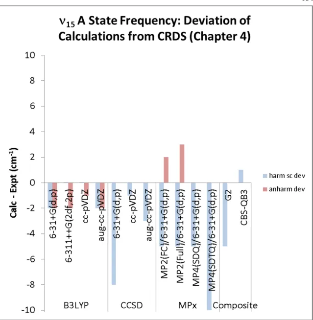
Figure 5.5. Deviation of calculated 15 A state frequency of HMP from experiment (CRDS from 15¹₀0⁰₀, Chapter 4).

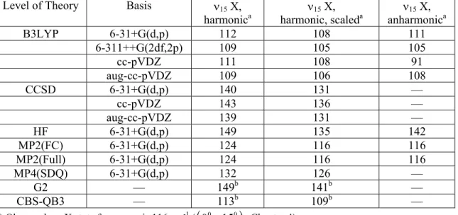
Table 5.4. Calculated 15 (OOCO torsion) frequencies (cm⁻¹) for the X state of HMP conformer A, harmonic, harmonic scaled,¹²⁸ and anharmonic.

Level of Theory Basis ₁₅ X, harmonic^a

₁₅ X,

harmonic, scaled^a ₁₅ X, anharmonic^a B3LYP 6-31+G(d,p) 112 108 111

6-311++G(2df,2p) 109 105 105

cc-pVDZ 111 108 91

aug-cc-pVDZ 109 106 108 CCSD 6-31+G(d,p) 140 131 —

cc-pVDZ 143 136 —

aug-cc-pVDZ 139 131 — HF 6-31+G(d,p) 149 135 142 MP2(FC) 6-31+G(d,p) 124 116 116 MP2(Full) 6-31+G(d,p) 124 116 116 MP4(SDQ) 6-31+G(d,p) 132 126 —

G2 — 149^b 141^b —

CBS-QB3 — 113^b 109^b — a) Observed ₁₅ X state frequency is 116 cm^-1 (



0⁰0151⁰



, Chapter 4)

b) Composite method frequencies taken from the zero-point energy calculation

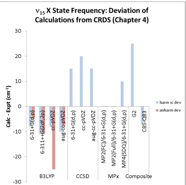
Figure 5.6. Deviation of calculated 15 X state frequency of HMP from experiment (CRDS from 0⁰₀15₁⁰, Chapter 4).

Table 5.5. Calculated 1 (OH stretch) frequencies (cm⁻¹) for the X state of HMP conformer A, harmonic, harmonic scaled,¹²⁸ and anharmonic.

Level of Theory Basis ₁ X, harmonic^a

₁ X,

harmonic, scaled^a ₁ X, anharmonic^a B3LYP 6-31+G(d,p) 3800 3663 3602

6-311++G(2df,2p) 3805 3676 3604 cc-pVDZ 3730 3619 3519 aug-cc-pVDZ 3783 3669 3580 CCSD 6-31+G(d,p) 3882 3626 —

cc-pVDZ 3840 3637 — aug-cc-pVDZ 3825 3622 — HF 6-31+G(d,p) 4175 3770 4001 MP2(FC) 6-31+G(d,p) 3859 3615 3667 MP2(Full) 6-31+G(d,p) 3861 3606 3669 MP4(SDQ) 6-31+G(d,p) 3886 3711 —

G2 — 4097^b 3864^b — CBS-QB3 — 3797^b 3672^b — a) Observed 1 frequency is 3622 cm⁻¹ (Chapter 4)

b) Composite method frequencies taken from the zero-point energy calculation

Figure 5.7. Deviation of calculated 1 frequency of HMP from experiment (CRDS, Chapter 4).

A-X transition frequency (Table 5.2, Figure 5.4) – Our desired accuracy for the calculated A-X bands is ±50 cm⁻¹. Based on the existing studies of alkyl peroxy electronic transitions, we expect that this level of accuracy for HMP will allow us to make predictions of larger systems (2-HIPP) within 100 cm⁻¹. According to Figure 5.4, CCSD (across three basis sets), MPx, and the composite chemistry methods all satisfy this requirement. B3LYP is only able to come within this accuracy using certain basis sets

(cc-pVDZ and aug-cc-pVDZ) or the time dependent formulation TD-B3LYP. We observe that CIS and TD-HF both predict the A-X frequency too low by 400 cm⁻¹, completely unacceptable.

15(A) torsional frequency (Table 5.3, Figure 5.5) – We immediately note that nearly all

of the methods tested can reproduce the 15 A state frequency to within 10 cm⁻¹, with the exception of HF/6-31+G(d,p). The majority of the calculated torsional frequencies are lower than the observed frequency (170 cm⁻¹). Overall, the B3LYP calculations are the most consistent and accurate (−2 cm⁻¹).

15(X) torsional frequency (Table 5.4, Figure 5.6) – In general, B3LYP (and even the

associated composite method CBS-QB3) and MP2 can reproduce the 15 X state frequency within 10 cm⁻¹. We see more signs of cc-pVDZ being too inflexible for modeling HMP: the B3LYP/cc-pVDZ anharmonic frequency is underpredicted by 25 cm⁻¹. Meanwhile, all of the CCSD calculations overpredict the torsional frequency by 15–20 cm⁻¹.

1(X) torsional frequency (Table 5.5, Figure 5.7) – CCSD does an excellent job of

modeling the OH stretch, reproducing the 1 frequency within 15 cm⁻¹ across all of the basis sets used. Scaled MP2 also is quite accurate. However, the anharmonic MP2 calculations, all B3LYP calculations, and the MP4 calculations perform poorly, with predictions off by at least 40 cm⁻¹.

Looking at all of the data in Tables 5.2–5.5 and Figures 5.4–5.7, we notice that each level of theory perform differently for each spectroscopic property. Table 5.6 summarizes which methods were considered acceptable for each spectroscopic band of HMP (A-X, 15 A, 15 X, and 1). Methods were considered acceptable if the results generally fit into the “acceptable range” (discussed above and listed in the table). There is no “perfect” method to model all four relevant bands. Nonetheless, with the exception of CIS and TD-HF calculations, reasonably accurate spectroscopic frequencies for HMP can be generated by using any of the quantum chemistry methods presented in this chapter.

Table 5.6. Summary of levels of theory that gave acceptable and unacceptable predictions of HMP spectroscopic bands

Band Expt. (Chapter 4) (cm^-1)

Acceptable range (cm^-1)

Acceptable levels of theory

Unacceptable levels of theory A-X 7391 ±100 B3LYP (Dunning)^a

CCSD MPx

TD-B3LYP G1/G2 CBS-QB3

W1

B3LYP (Pople)^a CIS TD-HF

15 (A) 170 ±10 B3LYP

CCSD MPx

—

15 (X) 116 ±10 B3LYP

MPx

CCSD

1 3622 ±20 CCSD B3LYP

MPx

a) Dunning type basis sets yielded errors of −65 and −73 cm⁻¹. Pople type basis sets yielded errors of −119 and −209 cm⁻¹.

Electronic, Torsional, and OH Stretch Frequencies for HMP Conformer B

We now turn our attention to HMP Conformer B, the second conformer that exists in a (relatively) deep potential well. We have not detected this conformer on our CRDS apparatus. Our calculations on this conformer serve as a prediction for future spectroscopic experiments.

We summarize the calculated A-X, 15 (A), 15 (X), and 1 frequencies in Table 5.7. We note that the A-X transition frequency for Conformer B is about 800 cm⁻¹ lower than Conformer A. This arises directly from Conformer B being higher in energy than Conformer A on the X state (600 cm⁻¹) and lower on the A state (−200 cm⁻¹), as observed in Figures 5.1–5.3. The vibrational frequencies for Conformer B are similar to Conformer A.

On the basis of Table 5.7, we estimate the A-X frequency to be 6600 ± 50 cm⁻¹,

15 (A) to be 170 ± 5 cm⁻¹, 15 (X) to be 105 ± 10 cm⁻¹, and 1 to be 3630 ± 20 cm⁻¹.

Table 5.7. Calculated A-X, 15 (OOCO torsion, A and X states), and 1 (OH stretch) frequencies (cm⁻¹) of HMP Conformer B. A-X scaled to HO2 (7029 cm⁻¹). Harmonic, scaled, and anharmonic vibrational frequencies reported.⁵⁴

Level of

Theory Basis A-X,

scaled ₁₅ A (harm/sc/anharm)

₁₅ X (harm/sc/anharm)

₁ (harm/sc/anharm) B3LYP 6-31+G(d,p) 6598 174 168 166 109 105 92 3813 3675 3617

6-311++G(2df,2p) 6590 174 168 170 109 105 92 3820 3690 3616 cc-pVDZ 6603 173 168 167 113 109 103 3760 3647 3567 aug-cc-pVDZ 6697 173 168 167 108 105 99 3798 3684 3606 CCSD 6-31+G(d,p) 6635 173 162 — 132 124 — 3888 3632 —

HF 6-31+G(d,p) 6361 179 162 174 154 139 146 4170 3766 3996 MP2(FC) 6-31+G(d,p) 6574 177 166 174 122 114 111 3868 3625 3680 MP2(Full) 6-31+G(d,p) 6574 178 167 175 123 115 112 3870 3615 3681

CIS 6-31+G(d,p) 6445 — — — — — — — — —

TD-HF 6-31+G(d,p) 6346 — — — — — — — — —

TD-B3LYP 6-31+G(d,p) 6548 — — — — — — — — —

cc-pVDZ 6607 — — — — — — — — —

Calculated Potential Energy Surfaces and Spectroscopic Frequencies of 2-HIPP

Finally, we extend the methods presented in this chapter to generate potential energy surfaces and to predict of the spectroscopic properties of 2-HIPP. 2-HIPP has a greater number of atoms (13 vs 7) and electrons than HMP (49 vs 33). At a given level of theory and basis, calculations on 2-HIPP will be more expensive than HMP. Because of this, we report less data for 2-HIPP than for HMP.

Figure 5.8 shows the X state potential energy surface for 2-HIPP as a function of the two dihedral angles OCOH and OOCO, at B3LYP/6-31+G(d,p), HF/6-31+G(d,p) MP2(FC)/6-31+G(d,p), and MP2(Full)/6-31+G(d,p). Figure 5.9 shows the A state surface of 2-HIPP at HF/6-31+G(d,p). Similar to Figures 5.1–5.3, all energies are in cm⁻¹, relative to the (OCOH, OOCO) = (0, 0) transition state.

Figure 5.8. 2-HIPP X State potential energy surfaces as a function of the dihedral angles

OCOH and OOCO. Surfaces calculated at B3LYP/6-31+G(d,p) (top left), HF/6-31+G(d,p) (top right), MP2(FC)/6-31+G(d,p) (bottom left), and MP2(Full)/6-31+G(d,p) (bottom right). Energies on the potential energy surfaces are in cm⁻¹, relative to the X state Cs

transition state energy.

2-HIPP X State B3LYP/6-31+G(d,p)

OCOO

-150-100 -50 0 50 100 150

OCOH

-150 -100 -50 0 50 100 150

0 500 1000 1500 2000 2500 3000

2-HIPP X State HF/6-31+G(d,p)

OCOO

-150-100 -50 0 50 100 150

OCOH

-150 -100 -50 0 50 100 150

-1500 -1000 -500 0 500 1000 1500

2-HIPP X State MP2(FC)/6-31+G(d,p)

OCOO

-150-100 -50 0 50 100 150

OCOH

-150 -100 -50 0 50 100 150

-500 0 500 1000 1500 2000 2500 3000

2-HIPP X State MP2(Full)/6-31+G(d,p)

OCOO

-150-100 -50 0 50 100 150

OCOH

-150 -100 -50 0 50 100 150

-500 0 500 1000 1500 2000 2500 3000

Figure 5.9. 2-HIPP A State potential energy surface as a function of the dihedral angles

OCOH and OOCO. Surface calculated at HF/6-31+G(d,p). Energies in cm⁻¹, relative to the X state Cs transition state energy.

Comparing the 2-HIPP surfaces (Figures 5.8 and 5.9) to HMP (Figures 5.1–5.3), we note several similar features. On the X state, there are three energy minima. The global minimum, equivalent to Conformer A, is off-axis, indicating that hydrogen bonding is leading to coupling of normal modes (although this coupling is not evident on the low-quality HF surface). The A state of 2-HIPP also has three minima. Similar to HMP, the global minimum of the A state corresponds to the equivalent of Conformer B.

The main qualitative difference between HMP and 2-HIPP are the energetics of Conformers B and C. In 2-HIPP, Conformer C is more stable than Conformer B (−200 cm⁻¹ for C vs 0 cm⁻¹ for B), and has a higher barrier to conformational change via the OOCO torsion (600 cm⁻¹ for C, 500 cm⁻¹ for B). In HMP, the opposite held true:

Conformer B was more stable energetically and had a higher barrier to conformational change.

2-HIPP A State HF/6-31+G(d,p)

OCOO

-150-100 -50 0 50 100 150

OCOH

-150 -100 -50 0 50 100 150

3500 4000 4500 5000 5500 6000 6500 7000

Table 5.8 summarizes calculated spectroscopic parameters of Conformer A of 2-HIPP: the A-X transition frequency (scaled to HO2), 33 (OOCO torsion) frequency in the A and X states, and 1 (OH stretch) frequency. These parameters were only calculated at selected levels of theory and bases due to the increased computational expense of 2-HIPP calculations compared to HMP. We note that at the most reliable levels of theory (B3LYP, G1, G2), the A-X transition is predicted to be in the range 7900–8000 cm⁻¹, well to the blue of HMP (7391 cm⁻¹). The B3LYP vibrational calculation predicts that the 1 band should appear in a similar location as HMP (3620 cm⁻¹), red shifted from a typical alcohol due to the internal hydrogen bond.

Table 5.8. Calculated A-X, 33 (OOCO torsion, A and X states), and 1 (OH stretch) frequencies (cm⁻¹) of 2-HIPP. A-X scaled to HO2 (7029 cm^-1).⁵⁴

Level of Theory

Basis A-X, scaled ₃₃ A (harm / sc)

₃₃ X (harm / sc)

₁ (harm / sc) B3LYP 6-31+G(d,p) 7913 132 / 128 113 / 109 3756 / 3621

HF 6-31+G(d,p) 7572 137 / 124 151 / 136 4168 / 3764 CIS 6-31+G(d,p) 7195 — — — TD-HF 6-31+G(d,p) 7204 — — — TD-B3LYP 6-31+G(d,p) 7362 — — — cc-pVDZ 7440 — — —

G1 — 7877 — — —

G2 — 7988 — — —

Discussion

Preliminary Thoughts on the Appropriate Level of Theory for Substituted Alkyl Peroxies The data presented in Figures 5.2–5.8 and Tables 5.1–5.9 show that no one single method can model all aspects of HMP accurately. Nonetheless, we can make preliminary

recommendations as to what methods should be used for modeling our HO2+carbonyl products on the basis of our HMP data.

Regarding the A-X electronic transition frequencies of HMP (Table 5.2, Figure 5.4), we note that CCSD, MPx, G2, and W1 perform similarly (within 50 cm⁻¹ of the observed value). However, the MPx surfaces (Figure 5.3) do not predict X state Conformer C to be bound, in contrast to all of the other calculated surfaces. Consequently, G2 cannot predict a transition frequency for Conformer C, since it uses an MP2 geometry for all of its energy calculations. ¹²³ At this time, we recommend CCSD or W1 for calculation of the A-X transition frequencies and potential energy surface calculations. Note that for larger systems such as 2-HIPP, these calculations will become very expensive, likely only accessible with a supercomputer. B3LYP can reproduce the qualitative features of the CCSD X and A surfaces and is much cheaper than CCSD.

However, the absolute accuracy of the A-X transition suffers (±150 cm⁻¹). B3LYP is likely an appropriate starting point for larger systems before embarking on the more expensive CCSD or W1 calculations.

Regarding the low lying OOCO torsional modes, we observe that B3LYP and MP2 are able to reproduce the frequency within 10% of the observed values. CCSD overestimates the 15 X state significantly (15%) across all of the basis sets used.

Although limited data exist at this time, we recommend B3LYP or MPx for calculation of torsional mode frequencies.

Regarding the OH stretch, only CCSD can consistently reproduce the observed frequency within 15 cm⁻¹. For B3LYP and MPx, the significant discrepancies between

the anharmonic and scaled harmonic frequencies raise questions about those methods’

accuracy. We recommend only CCSD for calculation of OH stretch frequencies.

Normal Mode Coupling and its Effect on Vibrational Frequencies, Sequence Bands The vibrational frequency analysis presented in Tables 5.2–5.5, 5.7, and 5.8 make use of the normal mode frequencies reported by Gaussian 09.¹²¹ The two torsional modes OOCO and OCOH are reported as pure torsions. However, the potential energy surfaces presented in Figures 5.1–5.3 show that the two modes should be coupled together due to the internal hydrogen bond. We therefore expect the actual vibrational modes to be mixed together, resulting in changes in the vibrational energy levels similar to HOONO (Chapter 3).

We also expect the internal hydrogen bond to affect the 1 spectrum. We may observe the formation of sequence bands due to torsionally excited HMP breaking the internal hydrogen bond, again similar to HOONO (Chapter 3). Unlike HOONO, this effect will likely not cause intensity to be shifted to the blue of the observed 1 band, because the frequency difference between HMP and similar alcohols is small (55 cm⁻¹, Chapter 4). Rather, we may observe significant sequence band formation to the red of the main band because the OH stretch frequency should decrease significantly as the geometry of HMP approaches the (OCOH, OOCO) = (0, 0) TS state, where there is even greater interaction between the OH and OO groups.

In order to fully understand how hydrogen bonding and coupling between vibrational modes affects HMP, we would have to explicitly calculate the energy levels based on the potential energy surfaces presented in this chapter. This study would be

interesting and worthwhile; we have already observed slight discrepancies in the width of the simulated and observed 1 spectra (Chapter 4). Unfortunately, such a project is outside the scope of our research, and would have to be performed in collaboration with a theorist (such as we did for the HOONO project in Chapter 3).

Conclusions

In this chapter, we have modeled spectroscopic properties of hydroxymethylperoxy (HMP) by computing the ground (X) and excited (A) state 2-dimensional potential energy surfaces as a function of the two dihedral angles (OCOH, OOCO), A-X electronic transition frequency, OOCO torsional frequency, and OH stretch vibrational frequency. Our potential energy surfaces reveal coupling between the OCOH and OOCO torsions on the X state (an effect of internal hydrogen bonding in HMP), but not in the A state. We locate three conformers of HMP on each surface, although the third conformer on the X state is either a shallow well or a shelf depending on the level of theory used. Our calculated electronic and vibrational frequencies are in excellent agreement with the experimentally observed HMP vibrational and electronic spectra (Chapter 4). On the basis of our results, we make the following recommendations for modeling our HO2 + carbonyl systems: CCSD for potential energy surfaces, CCSD or W1 for modeling electronic transitions, B3LYP or MPx for torsional frequencies, and CCSD for OH stretch frequencies. We applied these methods to 2-HIPP (HO2 + acetone) and predicted the A-X, OOCO torsion, and OH stretch frequencies. The torsion-torsion coupling observed on our X state surfaces indicates that explicit calculation of torsional energy levels may be required to accurately simulate HMP spectra.

Acknowledgements

We thank Heather L. Widgren for computing some of the G2 energies. The computations performed in this chapter were funded under NASA Upper Atmosphere Research Program Grants NAG5-11657, NNG06GD88G, and NNX09AE21G2, California Air Resources Board Contract 03-333 and 07-730, National Science Foundation CHE-0515627, and a Department of Defense National Defense Science and Engineering Graduate Fellowship (NDSEG).