We describe a technique for efficiently computing the dynamics of the dominant scale of a fluid system when only high-resolution simulation is available. The results include precise tracking of the dynamics of the dominant criterion for a range of parameter values for the computational superstructure.
Literature Review
Kevrekidis and colleagues (Theodoropoulos, Qian and Kevrekidis, 2000), who have continued to explore many elements and applications of coarse analysis. Gear (Gear and Kevrekidis, 2003a,b, 2004) focuses on the coarse analysis of systems described by ordinary differential equations.
The Coarse Analysis Framework
Kevrekidis has used the coarse integrator in calculating the evolution of system dynamics in many different applications (Gear and Kevrekidis, 2003a; Makeev et al., 2002b; Gear et al., 2002; Kevrekidis et al., 2003). Additional applications and analyzes of superstructure algorithms are provided in (Gear and Kevrekidis, 2003a; Kevrekidis et al., 2003; Li et al., 2003).
Coarse Timestepping
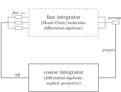
The coarse Euler timestepper shows that the detailed simulation is mainly used for extracting vector field quantities. The vector field is calculated using the detailed simulation over a burst time of h; therefore, a measure of the efficiency of the coarse algorithm is the ratio M/(k+ 1).
Numerical Analysis
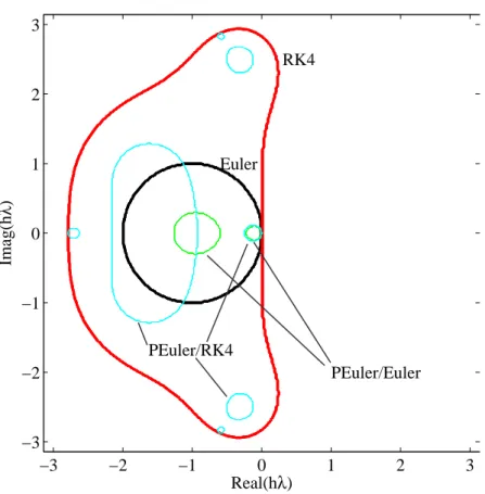
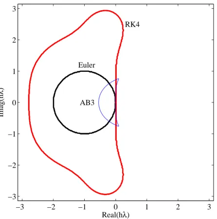
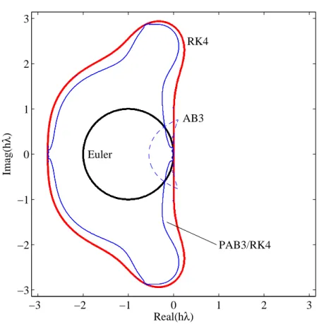
The regions of absolute stability are shown in Figure 2.3 for the Euler projective scheme where the detailed simulation is either itself an explicit Euler scheme or a fourth-order Runge-Kutta scheme. Note that for sufficiently high M/(k+1) ratios, the region of absolute stability for both designers.
Limitations and Challenges
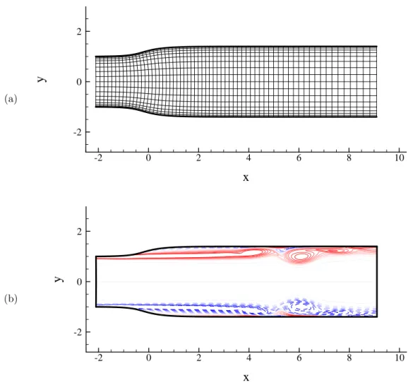
In this chapter we apply the coarse analysis methodology to extract the dominant features and the corresponding dynamics of the compressible flow in a planar diffuser. We provide an overview of the existing literature and known phenomenology for diffuser flows in Sections 3.1 and 3.2.
Literature Review
Steady injection applied from the centerline of the diffuser was implemented in conical diffusers by Nishi et al. Suzuki and co-workers have developed high-fidelity simulations for compressible diffuser flows (Suzuki and Colonius, 2003; Suzuki et al., 2004).
Diffuser Flow Phenomena
As the diffuser angle is increased, the diffuser action and the pressure gradients become increasingly severe, resulting in flow regime changes roughly in the order of the list given above. Multiscale descriptions For the large transient stall regime, in the case of planar diffusers, flow instability can be localized so that it occurs over just one side of the diffuser.
Equations of Motion
Furthermore, the spatial scales of the flow structures range between the smallest spatial scales, which represent the shear caused by the large eddy dynamics, and the largest scales, which are on the order of the diffuser length scales, represent the large eddies themselves. In this sense, diffuser flows in the large transient stagnation regime can be described as multistage flow systems.
Numerical Simulation
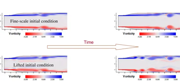
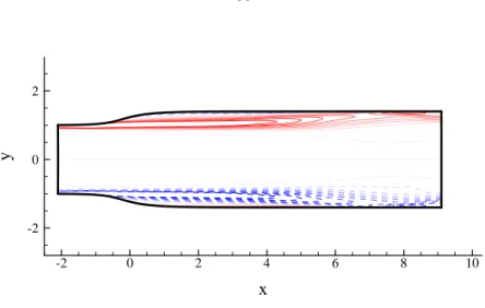
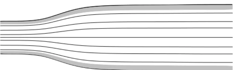
As shown in Figure 3.3, the multilevel nature of the fluid system arises from the eddy dynamics of the flow. The dominant dynamics of the system is related to the vortex dynamics of the large structures found in the flow.
Fluids: Coarse Analysis Using the POD for Scale Classifica- tiontion
This means that the POD coefficient vector gives a linear combination of the POD eigenfunctions that approximates the corresponding flow state. In other words, the lifting operator is a corresponding linear combination of POD modes where only the coefficients corresponding to the dominant scales are nonzero.
Coarse Time Stepping
A basic tool of coarse analysis is the coarse time indicator; this tool is used to calculate the time histories of the dominant rates. Therefore, before coarsening, it is the modified third-order Adams-Bashforth scheme for the dominant scales.
Numerical Analysis of a Coarse Adams-Bashforth Routine
Finally, note that the modified rough Adams-Bashforth scheme in Eq. 3.48) does not simplify to the rough classical scheme in Eq. 3.42), because the nature of the magnification differs for the schemes. Note that the right-hand side depends on quantities at time intervals not connected by 'detailed simulation'; that is, the right side is composed of three distinct portions near time indices n,n−M h, enn−2M h. The rough projective Adams-Bashforth scheme is stable for systems whose eigenvalues exist within the stability region.
Results: Coarse Diffuser Flows
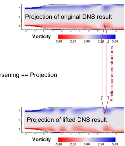
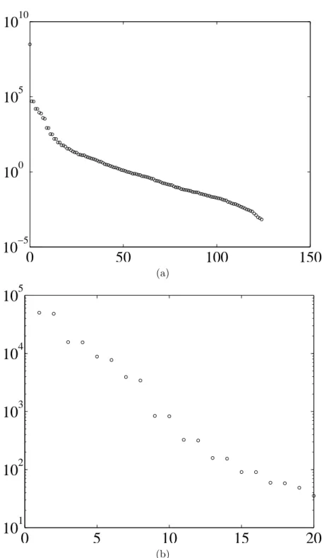
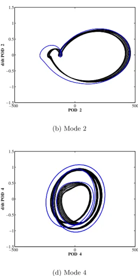
In Figure 3.13 we show the projections of the DNS simulation on the first twenty POD modes. We give a comparison of the original diffuser flow (calculated using DNS), projected into the first twenty POD modes, and the coarse numerical simulation in Figure 3.17. To clarify the coarse nature of the diffuser flow, a new coarse time integration is performed using .
Conclusions
In summary, we have shown that coarse analysis represents a promising alternative to the efficient, quantitative calculation of the dominant features of complex fluid flows. It is also important to note that the coarse numerical analysis outlined here for liquids involves the use of the correct orthogonal decomposition for scale classification. A comparison between coarse analysis and POD/Galerkin truncation can shed light on the shortcomings of the POD for scale classification and advan-.
Introduction
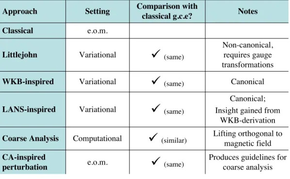
First, the detailed system, described by the Lorentz power law equations, is given in Section 4.2. The mean comparisons are then derived in two variational settings: one according to a WKB-style averaging procedure described in Section 4.5 and one according to a LANS-style averaging procedure described in Section 4.6. Numerical coarse integration is applied to the system and described in Section 4.7, and connections are made to perturbation theory in Section 4.8.
Lorentz Equations
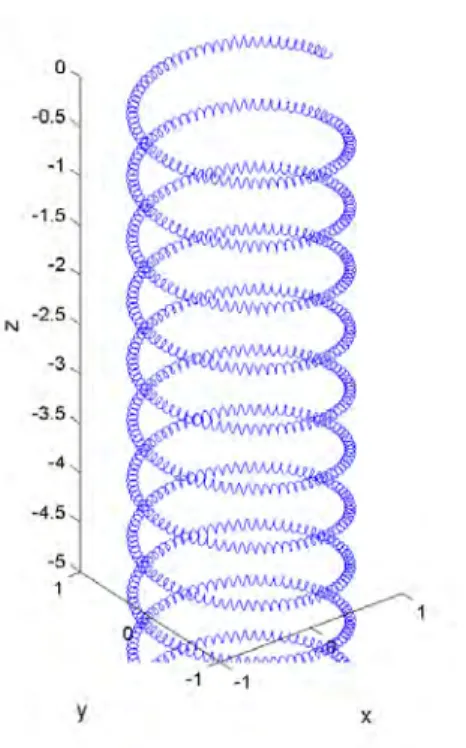
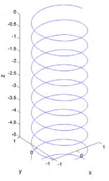
In this picture, the particle travels around the magnetic field with drift in the −ˆz direction. So the trajectories wind around the x-axis, which means that the motion is spiral around the magnetic field lines. The general outline of the magnetic field (with drift) represents the movement of the particle on a coarse scale.
Geometric Mechanics
Lagrangian Mechanics: Variational Principle For the Hamiltonian with canonical variables, the Legendre transformation can be applied to construct the Lagrangian for the system of charged particles. Using this, assuming that ∂A/∂t = 0, and applying the vector identities will lead to the Lorentz force law equation. Given this principle of action, the equations of motion for a charged particle in a magnetic field can be derived using a suitable action.
Guiding Center Equations
These equations, known as the governing center equations, describe the motion of the guiding center or the average position of the particles. The small scales of motion represent fluctuations in the motion of particles around the magnetic field; the average of these fluctuations isolates the movement of the leading center. For parameters and µ, these governing center equations govern the rough motion of a charged particle in a magnetic field.
Variational Averaging Inspired by WKB and Whitham Aver- agingaging
However, the equation is not closed in the sense that a dependence on the fluctuations remains. To investigate this dependence, we derive the corresponding Euler-Lagrange equations by considering variations in the fluctuations qf:. With b=B/kBkthe unit vector in the direction of the magnetic field we can use Eq. rewrite.
Variational Averaging Inspired by LANS Averaging
These terms correspond to terms appearing in the WKB/Whitham-style mean Lagrangian given in Eq. Note that in the WKB/Whitham-style derivation this term is ignored once the scaling assumptions in Eqs. The idea behind this choice is that in the WKB/Whitham context xf and yf are the cos and sin components of the fluctuation, respectively.
Coarse Timestepping
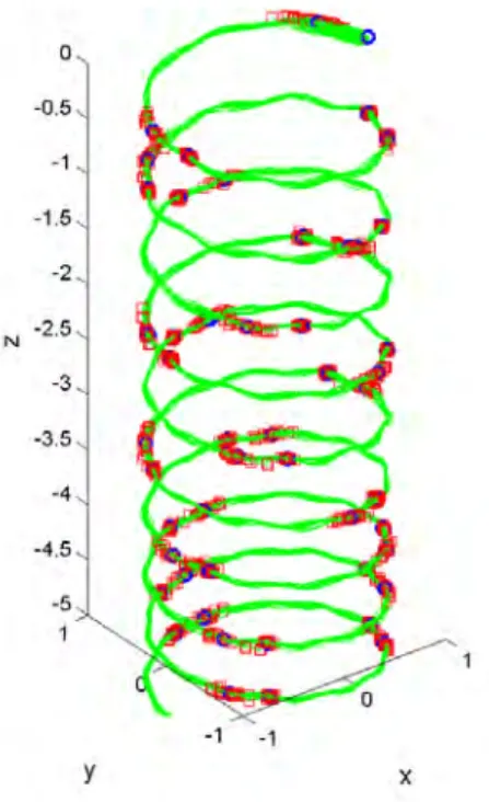
Because this is a small system of ordinary differential equations, and because no projective time integration scheme is used, there are no computational savings from using the coarse integrator. Note that this coarse integrator was able to calculate the coarse dynamics for a Hamiltonian system. This may or may not be valid, depending on the type of trajectories and averaging and on the underlying structure of the dynamical system.
Lifting and Averaging
We want to compare ψ with the flow mapψGC for the leading central vector field. To put this in the context of coarse analysis, we note that we can now approximate the leading vector field at the center by choosing an appropriate lift and mean map and applying it to the original vector field for the Lorentz force system . Because this represents another relationship between averaging and the equations of motion, we now consider derivations of the leading center equation using techniques that allow approximations.
Hamiltonian Averaging
Here, we have assumed that averaging and calculating the Hamiltonian motion, and there are additional assumptions related to the action of the operator ∇ and the chain rule. We seek to demonstrate that this expression is equivalent to the expression for the mean vector field. This means that this mean vector field ¯X, which is Hamiltonian, corresponds to a map of the mean flow of the system.
Conclusions
Because of the success of the averaging theory in deriving center-of-direction approximations to the original Lorentz force system, the application of coarse analysis to this conservative system is considered. To this end, averaging techniques influenced by coarse analysis are applied to the equations of motion for the charged particle system. Using the POD as a scale classification allows us to implement coarse analysis techniques.
Objective
Implicit Finite-Difference Schemes
For the diffuser code, α is set to 1/10, we arrive at the classical fourth-order Pad´e scheme.
Explicit Finite-Difference Schemes
Sixth-order centered difference We repeat the procedure for the first derivative case, except now R. Third-order upward difference We repeat the procedure for the first derivative case, except now R=. Upward (forward) difference of the fourth order We repeat the procedure for the first derivative case, except now R.
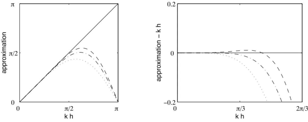
Optimized Spatial Discretization
The finite difference scheme can then be optimized in the sense that the error between Etussen the wavenumber and the effective wavenumber is a minimum. A comparison between the optimized scheme and the standard fourth- and sixth-order finite difference schemes is shown in Figure A.1. A comparison between the optimized scheme and the standard fourth- and sixth-order finite difference schemes is shown in Figure A.2.
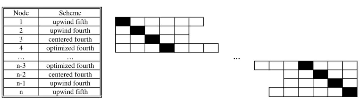
Implementation
The primary scheme is sixth-order Pad´e, and the terminal node scheme is up (explicitly) third-order. For greater accuracy, longer templates are used for end knots; the shorter templates used at the end nodes resulted in instability and the appearance of spurious modes for this study.
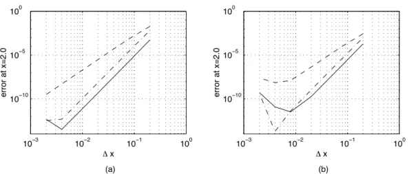
Error Analysis
From Figure A.6, it is evident that the full Pad'e and explicit/cross-stream Pad'e schemes calculate the lowest residuals compared to the other cases. Also note the high correlation between full Pad'e and explicit/transverse Pad'e calculations. This explicit/transversal Pad'e formulation will be used for future parallel implementations of the hub code, as the formulation explicitly accepts a parallel domain partitioning framework.
Concluding Remarks
Parallelization was performed according to the Message Passing Interface (MPI) standard because of the popularity and ease of use of MPI in applications that require distributed processing or memory.
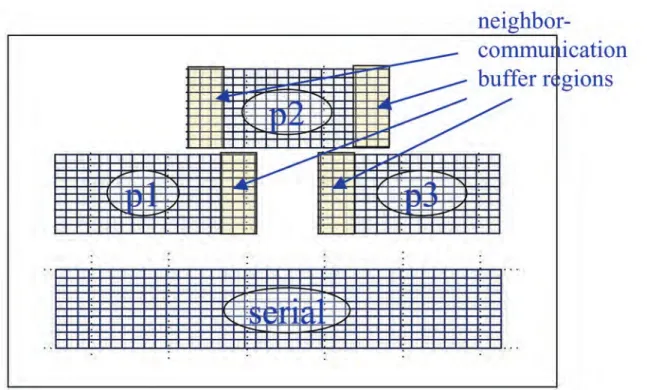
Domain-Splitting Framework
Each processor must communicate information about the boundaries of its local domains to maintain continuity in computing flow physics. As shown in this figure, the local domain for each processor is expanded so that processors responsible for adjacent regions can communicate their boundary information. There are communication and computation costs associated with calculating the flow in these communication areas.
Setup: the mpi basic Module
The algorithm is very simple and can exhibit pathological behavior depending on the domain size; investigate this subroutine if the calculated local domain sizes are nonsensical. Please note that padding is only added to the local domain boundaries that do not coincide with the global domain boundaries. The following code documents this algorithm and the definition of the variables mpi imin and mpi imax for the domain local to the processor.
Communication: the mpi advanced Module
In this routine, the processor first posts a send message to processor+ 1, and then the processor posts a receive message to processor+ 1. The arguments are as follows: qtemp(1) refers to the address of the first value in qtemparray;. Note that, as a complement to the NandNminus1(q, nvars) thread transfer routine, the processor first posts an acknowledgment to processor-1, and then the processor sends a dispatch to processor i-1.
Specifics
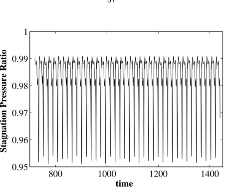
Algorithms for calculating stagnation pressure ratios and skin friction are included in a later subsection. Revisions in the ddt module The stagnation pressure ratio and skin friction routines have been converted to distinct subroutines (the prcv calculation and cf calculation subroutines, respectively) within the ddt module. Only the processors responsible for calculating the stagnation pressure ratio are active in this subroutine.
General Revisions to the diffuser Code
Results
Comparision with Serial diffuser Results
Benchmark Timing Study
Program Compilation and Execution
Bugs