Many thanks to all the colleagues in the office for helping me with different types of processes, for example with expense reports. I would also like to thank all my fellow graduate students who made my post-graduate life possible.
Introduction
Dehn surgery of 3-manifolds
Group theoretic Dehn fillings
By considering Dehn fillings of hyperbolic nested subgroups [13] constructs pure pseudo-Anos normal subgroups of mapping class groups. Recently, Dahmani-Guirardel-Osin [13] proved an analogue of Thurston's theorem in the more general setting of groups with hyperbolically embedded subgroups (see Theorem 1.1.4 below and the discussion following it).
Motivation: a question on group cohomology
Thurston's geometrization conjecture, proved by Perelman, implies that this algebraic statement about π1(M(s)) is equivalent to the hyperbolicity of M(s). Note that in the settings of Thurston's theorem, ie. if G=π1(M), H =π1(∂M) and M(s) admits a hyperbolic structure, we have.
Main results
- Cohen-Lyndon type theorems for hhN ii
- Structure of relative relation modules
- A spectral sequence for Dehn fillings
- Homological properties of Dehn filling quotients
- Quotients of acylindrically hyperbolic groups
For general hyperbolically embedded subgroups, a weak version of the Cohen-Lyndon property is given in [13, Theorem 2.27]. For acylindrical hyperbolic groups, [13, Theorem 6.14] construct hyperbolically embedded subgroups of the form described in condition (b).
Words and Cayley graphs
In Sections 2.5 to 2.7, whose main references are [13, 29], we recall the definition and basic information about cylindrically hyperbolic groups and (weakly) hyperbolic embedded subgroups. In Sections 2.6 and 2.7 we review the concepts of isolated components and diagrammatic operations introduced by Osin [27] and useful in the proof of Cohen-Lyndon type theorems in Chapter 3.
Van Kampen diagrams
In the following, the above assumptions (c) and (d) will be imposed on the van Kampen diagrams. The well-known van Kampen lemma states that a wordwoverRepresents1inGif if and only if there is a van Kampen diagramΔover (2.1) such that ∆ is homeomorphic to a disc (such diagrams are called disc diagrams), and thatLab(∂∆)≡w.
Gromov hyperbolic spaces and Gromov boundary
If a van KampenΔ diagram is homeomorphic to a disc, and O is a vertex of i∆, then there is a unique continuous map µ from the 1-skeleton of i∆ to the Cayley graphΓ(G,A) sending O to the identity vertex, preserving the labels of core edges and non-core edges collapsing into points. The elements of ∂Se are just equivalence classes of Gromov sequences in Sand and we say that a sequence{xn}n>1 ∈S tends to the limit pointx∈∂See and writexn→ x asn→ ∞if{xn}n>1∈x.
Acylindrically hyperbolic groups
Hyperbolically embedded subgroups and group theoretic Dehn fillings
We say that {Hλ}λ∈Λ is weakly hyperbolically embedded in (G, X)(denoted as {Hλ}λ∈Λ,→wh(G, X)) ifGis generated by the setXtogether with union of allHλ, λ∈Λ , and the Cayley graphΓ(G, Xt H) is a Gromov hyperbolic space. One remarkable property of weakly hyperbolically embedded subgroups is the following group-theoretic Dehn filling theorem.
Isolated components
ToHλ componentsq1, q2ofpair called connected if there exists a sticinΓ(G, Xt H) such thatc connects a vertex ofq1 to a vertex ofq2 and that Lab(c) is a letter from Hλ. There exists a positive number satisfying the following property: Letpbe ann-gon inΓ(G, Xt H)with geodesic sidesp1, .., pnog letI be a subset of the set of sides of such that each sidepi ∈Iis an isolated Hλi- component of pfor someλi ∈Λ.
Diagram surgery
If there is a diagram∆∈ D such that ∂ext∆≡w, by filling the holes in ∆s with faces whose boundaries are denoted by words from S, we create a circular van Kampen diagram over (2.2) whose boundary is denoted by w. Then there exists λ∈Λ and a connected componentof∂int∆such that it is connected to the Hλ-component of ∂ext∆.
Direct sums and products of abelian group homomorphisms
An Hλ subpath p of ∂∆ (resp. ∂∆) is called an Hλ component if p is not properly contained in any other Hλ subpath.
Chain complexes
Resolutions and Ext functor
It is well known that the Ext groups given by the above two definitions can be naturally identified (for example, see [31, Theorem 7.8]). Further, if M0 → I0 is an injective resolution over R0, then M → M0 induces a chain mapping from M → I to M0 → I0, which further induces a chain mapping.
Group cohomology
But in the case of computations, we might have to use the solution P → S (resp. M → I) and thus write H∗(HomR(P, M))(resp. A standard fact in group cohomology is that the modular structure onExtK(A, A0 ) does not depend on particular choices of projective solutions (see e.g. [10, Chapter III.8]).
Coinduced modules
A generalization of Shapiro’s lemma
It is easy to see that Shapiro's Sha isomorphism is a chain isomorphism and thus induces an isomorphism between cohomology groups.
Group triples and Cohen-Lyndon property
Hλ :Hp(G;Hq(hhN ii;A))−→Hp(Hλ;Hq(Nλ;A)) be the natural map corresponding to the natural homomorphismHλ →GandN T RqN. A group triple(G,{Hλ}λ∈Λ,{Nλ}λ∈Λ) has the Cohen-Lyndon property if there exists a left transversalTλ ∈LT(HλhhN ii, G) for everyλ∈Λ such that.
Spectral sequences of cohomological type
A group homomorphism :A → B is called amorphism between bigraded abelian groups of bigrad(k, `)for somek, `∈Ziff(Ap,q)⊂Bp+k,q+`for allp, q∈Z. Assume that Ei ={(Ei,r, di,r)}r>a(resp.Hi),i∈I, forms a directed system of spectral sequences (respectively graded abelian groups).
Cartan-Eilenberg resolutions
For each p, q∈Z,hZp,q(resp.hBp,q,hHp,q) is called the horizontal concurrence (resp.horizontal coboundary, horizontal cohomology) of Iat position(p,q). Moreover, the notation(I,hδ,vδ)−→f (C, d)(or briefly I −→f C, I →C, etc.) indicates thatI is a CE resolution of Canf the magnification. After the proof of Theorem 3.0.1, we will discuss the application of the Cohen-Lyndon property to relative relation modules.
Construction of the transversals
Let W be the set of collections{Wλ}λ∈Λ of words satisfying (P2) and (P3), while instead of (P1), we only require that the words in Wλ represent a subset of a transversal inLT( HλhhN ii, G) for each λ∈Λ. We order W by indexical inclusion, i.e. {Uλ}λ∈Λ is less than {Vλ}λ∈Λif and only ifUλ ⊂Vλfor everyλ∈Λ.W is nonempty because the collection{Wλ}λ∈Λwith eachλ consists only of empty words is member of W. Assume that {Tλ}λ∈Λ does not satisfy (P1), i.e. there existsλ0 ∈Λ andg ∈ Gsuch that no element in cosetgHλ0M is represented by a word inTλ0.
If Contains at least one letter from, then can be decomposed as w ≡ uhhow ath ∈ Hλ\{1}for someλ∈ Λandv does not contain letters from H(u, item must be empty words).
Proof of Theorem 3.0.1
By Lemma 2.7.8, there exists λ ∈ Λ and a connected component c of ∂int∆ connected to an Hλ component of ∂ext∆. Ifpni is connected to an Hλi component ofpti+1, thenti+1 can be decomposed asti+1 ≡ uhvwithh∈Hλi\{1}(u, item must be empty words),ti≡u, anddbλi(1, nih)>12D . Ifpni is connected to an Hλi component of pti+1, then ti is equal to some prefix of ti+1, by Lemma 3.2.13.
By Lemma 3.2.12 there is only one possibility for this case: j =i+ 1,pni is connected to an Hλi component of pti+1, andpni+1 is connected to anHλi+1 component of pt−1.
Relative relation modules
For proof, one must join the Hλk components associated with it in the construction of p, and sharpen the approximate estimate (3.6). Let G be a graph of groups, letπ1(G) be the fundamental group of G, let {Gv}v∈VG be the collection of vertex subgroups, and let {Ge}e∈EG be the collection of edge subgroups. Let G be a graph of groups, letπ1(G) be the fundamental group of G, let {Gv}v∈VG be the collection of vertex subsets, and let {Ge}e∈EG be the collection of edge subsets.
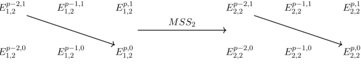
More precisely, we consider M SS :EG → EH as a morphism of the spectral series (1.2) to EH and we have a commutative diagram forr >2:.
Idea towards proving Theorem 1.2.10
Isomorphism of iterative cohomology groups
We use the notation defined in notation 2.14.2. N1) for allλ∈Λ,Hλ∩ hhN ii=Nλand thus a natural homomorphism. It is easy to check that SCHλ is well defined, i.e. independent of the choice of representative fbo of the cohomological class[fb]. As aZHλ-module, ZG is freely generated by z ∈ S and thus we can ZHλ-linearly expand Fb to a function (still denoted by).
As a ZHλ module, ZG is freely generated by s∈S and so we can expand ZHλ-linearly to a function (still denoted by).
Proof of Proposition 4.2.3
It follows that Rλ for every λ∈Λ is a free ZhhN ii-module, since it is the direct sum of free ZhhN ii-modules. Since none of the factorizations x1 and x2 ends with a factor from Nλt1, the only possibility for x−11 is x2∈Nλt1 x1 =x2. The mappings F gλ and 0λ are homomorphisms of the ZhhN ii-module, and right multiplications are automatically homomorphisms of left modules.
Note that e(Re1) is aZhhN ii submodule of ZhhN generated by elements of the formxnt−xwitht ∈ Tλ, x∈ Xλ,t, n ∈ Nλ, λ ∈ Λ, and thus (Re1) is the augmentation ideal of ZhhN ii.
Proof of Proposition 4.2.1
Morphisms of Lyndon-Hochschild-Serre spectral sequences
Lyndon-Hochschild-Serre spectral sequences
The LHS spectral sequence for (G,hhNii, A) is the spectral sequence {(hEG,r,hdG,r)}r>2 which resulted from deleting the E1 page of hEG. There is no essential reason for removing the E1 page in the construction of LHS spectral sequences. We follow this approach only because it simplifies the construction of spectral order morphism in the proof of Theorem 4.0.1.
The LHS spectral sequence for (H, N, B) is the spectral sequence {(hEH,r,hdH,r)}r>2 resulting from deletion of the E1 side of hEH.
Let M SSλ,rp,0 be the composition. the definition of M SSλ,rp,0 does not depend on the choice of R). By successively applying Lemma 5.1.6 (with pin-site of p−1i part (a)), we see that M SS2p,0 is surjective and thus is an isomorphism. Thus, the five lemma implies that the last vertical map of (5.15) is also an isomorphism.
Let {x, y, t} be a free basis of F3, let {ci}i∈I be a generating set of C, and letwi, vi, i∈I, be freely reduced words over the alphabet {x, y} such. a) the wordsciwi, i ∈ I, satisfy the condition of small cancellation C0(1/2) on the free product hxi ∗ hyi ∗C;.
Proof of Theorem 4.0.1
By restricting the domain of this morphism to EG and the target of this morphism to EHλ, we obtain a morphism. It is easy to check whether M SSλ,r, r>2, constructed above, forms a morphismM SSλ :EG → EHλ between spectral sequences. For q = 0 andp ∈ Z it is well known that H0(hhN ii;A) can naturally be identified with thehhN ii- fixed points ofA, and forλ∈Λ,H0(Nλ;A) can naturally be identified with theNλ- fixed points fromA.
In this chapter, we first perform calculations with spectral sequences to extract certain information from such a morphism.
Computations with spectral sequences
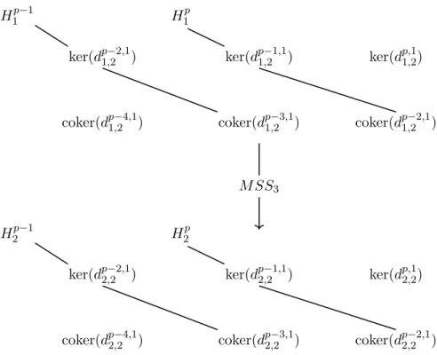
The only possibly non-trivial differences on the second page of E1 or E2 are the differences that go from the first row to the 0th row. After completing the calculations on the second page, we get the third page, which is shown in Figure 5.2. Similarly, other line segments in Figure 5.2 indicate different consequences of the boundaries of E1 and E2. Since fp is an isomorphism and M SS is compatible with fp, comment 2.15.11 implies that M SS2p,0 is an isomorphism.
Cohomology of Dehn filling quotients
Thus, the top horizontal map of (5.12) is also an isomorphism, which proves that lim−→M SSi,2p,1 is an isomorphism for p>1. Taking the direct limit of (5.16) and using the fact that lim−→is an exact functor, we obtain the following. By Theorem 5.2.5 and the assumption that F is of type F P∞, the last vertical map of (5.17) is an isomorphism.
The five lemma therefore implies that the second vertical map of (5.17) is also an isomorphism, which proves that lim−→M SSi,20,1 is an isomorphism.
Cohomology and embedding theorems
Assume that G, Hλ, λ∈Λ, are of type F P. If one of the following conditions holds for each λ∈Λ, then Gal is also of type F P. F2) Hλ is of the form Kλ×Fλ, where Kλ is finite and Fλ is a finite rank free group and Nλ6Fλ. It follows from Greendlinger's lemma for free products [24, Chapter V Theorem 9.3] that if kwik,kvik, i∈I, are sufficiently large, then Q is injective onF and thus (2) is guaranteed. If C is of type F P∞, then C is finitely generated and we can construct using a finite generating set of C, i.e. map(I)<∞.
Note also that it is the free product of a free group of finite rank F3 withCand thus of type F P∞.
Common quotients of acylindrically hyperbolic groups
According to (NT1), each subword of the first type has a length of at least 1, and thus the total length of the subwords of the first type is at least n. Then there are four consecutive components of p which are related to four consecutive components of q. We observe the following estimate of the length of the longest subword Lab(r)over{ck+1, ck+2}.
Arguing as in Case 1.1, we see that there are aG10-componentfulfillment and aG10-component0many sharing the same endpoints.
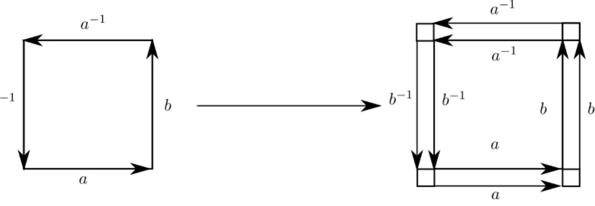
How to produce a cut system
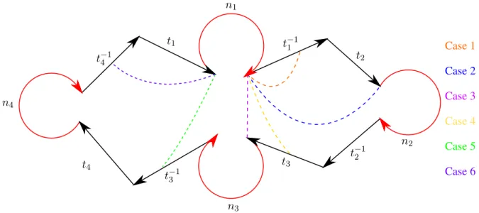
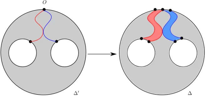
An illustration of Case 1 in the proof of Lemma 3.2.7
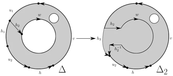
Cases 1 through 6 in the proof of Lemma .12
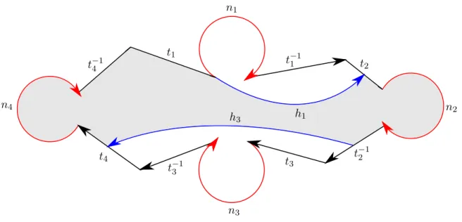
The construction of p
The second pages of E 1 and E 2
The third pages of E 1 and E 2