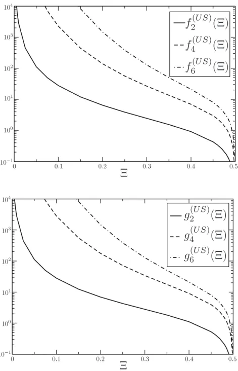
211 I.4 The fall speed of square grids with varying grid spacing S and position across the channel. 212 I.5 The fall speed of square grids with varying grid spacing S and position across the channel.
A model system from continuum mechanics
In the limit that the material is incompressible, so that the isothermal compressibility and isobaric expansion of the fluid are small, the density is effectively constant and the velocity field is divergence-free. This thesis is concerned with low Reynold number flows, such that viscous forces throughout the fluid are significantly stronger than inertial forces, so the limit that Re→0 is considered.
The Green’s function formulation for Stokes flow
This is the basic solution for Stokes flow such that, for an arbitrary body force on the fluid denoted f(x), the resulting flow is Here, P(x,x0) is the Green's function for the pressure field in Stokes flow and δij is the Kronecker delta function.
The grand mobility tensor
The inverse of the large mobility tensor is called and denoted the large resistance tensor. In fact, the calculation of the former quantity is at the heart of the calculation problem.
The Langevin equation
This convention is adopted throughout the manuscript and is easily recognizable by the complete absence of statements regarding torque and rotational speed. The last term reflects the implicit dependence of the Brownian forces on the particle configuration.
Stokesian dynamics
Computationally, this "deterministic drift" is the result of using a low-order integration scheme that does not account for the intermediate particle configurations that must occur as a particle translates over a single time step. With some algebraic manipulations, this system of equations can be solved for the far-field hydrodynamic force and the particle velocities as
Model systems
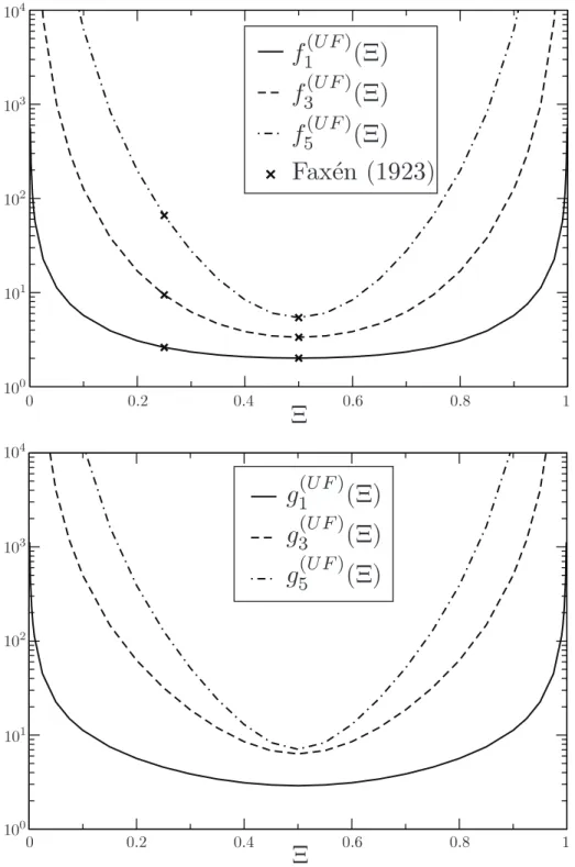
This is the tension caused by the deformation of a sphere near a plane wall - one of the main quantities for determining the stress in a suspension of spheres. The method of separation of variables in bi-spherical coordinates is used to calculate these quantities as a function of the distance between the particle and the plane wall.
Analysis
Axisymmetric motion
For the rotation of a spherical particle about the axis perpendicular to a nearby wall, the drag torque is equal to the torque on the particle. Similarly, for a spherical particle that translates to a nearby wall, the drag torque with the force on the particle is the same.
Transverse motion
Recall that it is the coupling between the deforming contribution to the shear flow and the moments of force that includes RF E, RLE and RSE. Note that these terms corresponding to the deformation can actually be written in terms of a rotation (the first term) and a second inhomogeneity.
Lubrication expansions
Results
While there is sufficient information in ˆF and ˆL to calculate strain coupling constants, the quantitative accuracy of the present results can be assessed by comparison. This serves as an indirect verification of a completely new stress-strain coupling calculation.
Conclusion
Although others have developed simulations of colloidal particles near a single wall, these studies lack a key symmetry of the method here [Bossis, Meunier and Sherwood (1991), Jendrejack, et al. 2004)] or the physical and mathematical simplicity of the original Stokes dynamics technique [Cichockiet al. Examples are given to illustrate the importance of the symmetry of the drag and mobility tensors.
Analysis
The same Fourier transform approach that was used to calculate Blake's expression for the reflection of Stokeslet (Jw(x,y;H)) can be used to calculate the reflection of the source doublet [Blake and Chwang (1974)]. If we know the reflection of the Stokeslet that satisfies the boundary conditions on the wall, then we can calculate the perturbation velocity generated by a particle with an arbitrary force density using the procedure just described.
Results
Symmetric mobility and resistance tensors
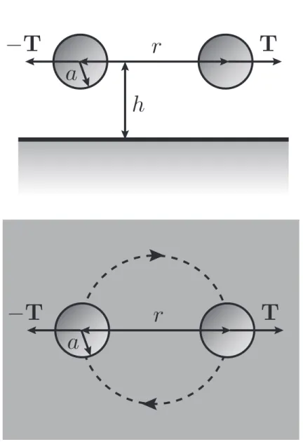
Co-rotation of a doublet of particles
Since the torques on the particles are equal and opposite, the doublet is a force- and torque-free object. The only difference between the doublet and the bacteria is that the bacteria is also driven along its centerline.
Grand mobility tensors for any confining boundaries
However, Green's function in this case is a linear combination of Green's functions for a free surface (GF(x,y;H), eq. 4.19) and a solid plane wall (GW(x,y;H), cf. Taking the same linear combination of the large mobility tensors for particles near a free surface and particles near a plane wall, the large mobility tensor for particles near a liquid-liquid interface is obtained.
Conclusions
Other approaches to calculating channel mobility have similar characteristics (Ganatos et al., 1980: boundary collocation method). A number of researchers have made experimental measurements of the in-plane diffusivity of a particle between parallel walls. We introduce the Fourier transform solution to the Stokes equations between parallel walls and demonstrate that this can be used to develop an integral expression for components of the large mobility tensor for a single particle in a channel.
Analysis
- The grand mobility tensor revisited
- General solution to the Stokes equations between parallel walls
- Single particle mobility in a channel
- Stokesian Dynamics revisited
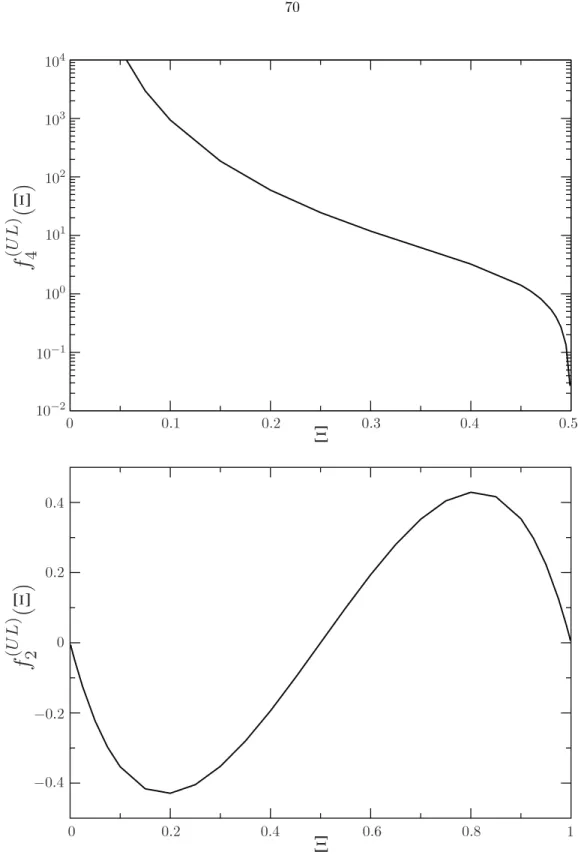
This is the mobility tensor MU F for a particle in a channel, and similar expressions can be developed for the other parts of the large mobility tensor (see Swan and Brady, 2007). These are now complicated functions of the mutual coordinates (k1, k2), the distance between the plates (H) and the fractional distance across the channel (Ξ). Likewise, so are the elements of the large mobility tensor for the rotation-torque and rotation-stress couplings.

Results
Components of the single particle mobility in a channel
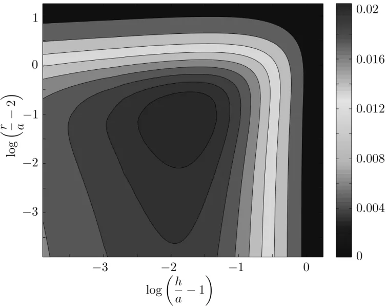
These results are easily recognized as the coefficients of the single-wall mobility tensor (Swan and Brady, 2007), which is sometimes written as. For a particle above a single wall, the torque is also linked to the translation of the particle. When translated perpendicular to the walls, the error is almost 60 percent in the center of the channel.
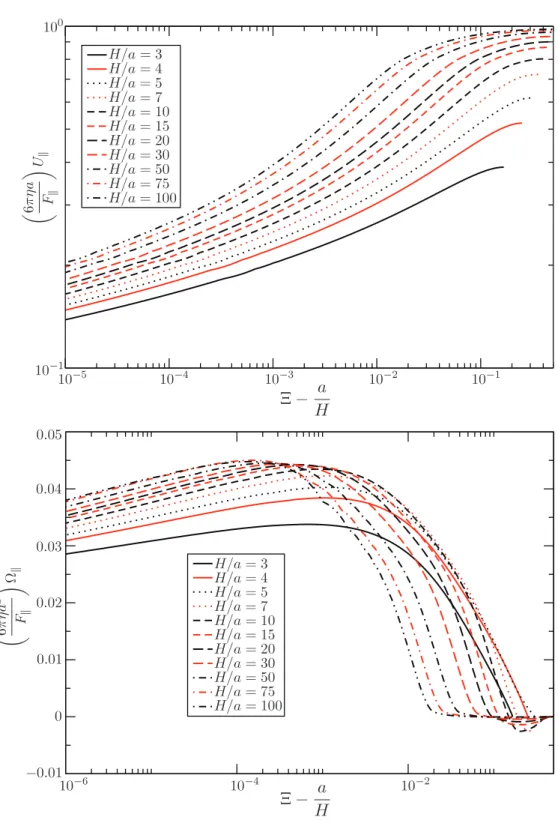
Sedimentation of a particle between parallel walls
Of particular interest is the fraction of the channel over which the sedimentation rate is close to the mid-channel rate. We use this to calculate the fraction of the channel over which the mean particle fall velocity is greater than 95% of the mean channel fall velocity. We expect that as the channel becomes wider, the portion of the channel where sedimentation is close to the mid-channel velocity will increase monotonically.
Brownian drift of a particle in a channel
Einstein viscosity for a dilute suspension between parallel walls
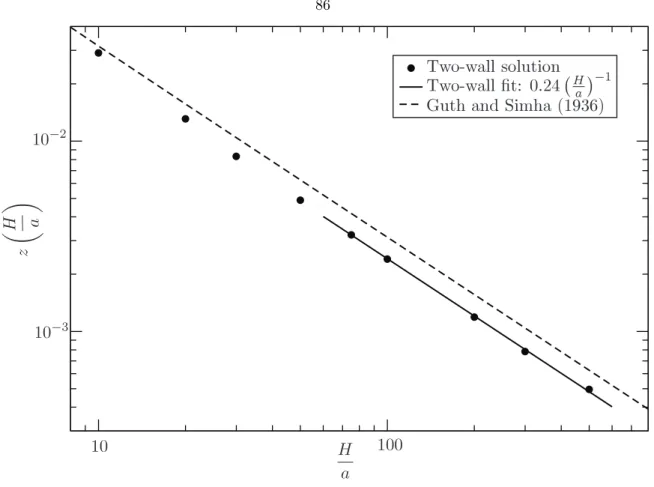
Shortly after Einstein made his calculation of the viscosity of a dilute suspension, Guth and Simha (1936) attempted to include the effects of channel walls on the viscosity of the suspension. In Figure 5.13 we plot the additional contribution to the viscosity of a dilute suspension as well as the result due to Guth and Simha. That the viscosity calculated via superposition is greater than that due to the exact two-wall solution to the Stokes equations is perhaps most easily understood by analogy.
Conclusions
All higher-order reflections arose from a multipole expansion of the frontier integral solution of the Stokes equations. Durlofsky and Brady (1989) combined their Stokesian Dynamics algorithm with a discretized model of the channel walls that takes into account the additional energy dissipation due to the anti-slip condition on the walls. Another approach comes from Staben et al. 2003) relies on the boundary integral formulation for Stokes flow and uses the Green's function for channel flow [Liron and Mochon (1976)] in the calculation of the hydrodynamic resistance to particle motion in a canal.
Analysis
- Stokes flow in a channel subject to an arbitrary, periodic body force
- The Ewald summation technique
- Reflections in real-space
- Computations in wave-space
- Simulation methods
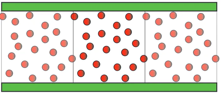
When the Fourier coefficients of the stress in the fluid are denoted as σ(k)(x3), the total force on the channel walls in one period is the same. In this case, the distance of the source from the wall (indicated by a thick line) is p. It is undesirable to repeat the calculation of the wave space contribution to the current felt by each particle.

Results
- Cooperative motion of regular lattices
- High-frequency dynamic viscosity
- Short-time self-diffusivity
- Sedimentation rate
In particular, one is interested in the response to a shear flow created by the differential translation of the channel walls. Moreover, there is a weak dependence of the sedimentation rate on the channel width in the low volume fractions. Furthermore, the sedimentation rate profile along the channel shows an interesting dependence on the volume fraction.

Conclusions
In an experiment, the autocorrelation in time of the intensity of the laser light scattered by the suspension is measured. An extensive study of the relationship between local suspension density fluctuations and its short-term dynamics was conducted by Rallison and Hinch (1986). Similarly, Brady (1994) continued this line of research in his search for long-term suspension dynamics.
Analysis
Statistical theory
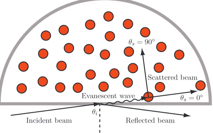
This effective wave vector will prove to be particularly convenient for linking the light scattering experiments with the dynamics of the suspension. Recognize that the integrand of the zero-time self-intermediate scattering function is a probability density weighted by the exponential decay of the evanescent wave. The difference here is the introduction of an exponential weighting of the averages caused by the decay of the evanescent wave.
Simulation methods
However, in the far field the hydrodynamic interactions have a large range (scaling such as r−2 in the presence of a macroscopic boundary, where r is the distance between particles). Similarly, we refer the reader to the companion paper by Swan and Brady (2010), which describes in detail the modeling of the hydrodynamic interactions between many particles in a suspension between macroscopic boundaries. This provides the opportunity to actually multiplex the data by considering the hypothetical situation in which evanescent waves originate from both the upper and lower walls of the channel.
Measurement techniques
- Static measurements
- Dynamic measurements
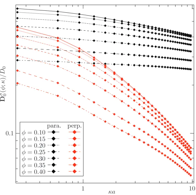
For example, DkS(φ, κ) is the ensemble average of the velocity of one particle parallel to the wall due to the force on that particle only in the same direction and magnitude exp(−κz) divided by the average exp(− κz) where the height of the particle above the wall, i.e. Considering that the Brownian trajectories of the particles are known, we try to measure the intermediate scattering function for a given penetration depth and thus the evanescent diffusivity. It is clear that the time derivative of the logarithm of these functions at t = 0 are the evanescent diffusivities.
Results
In the limit of the large scattering wave vector, the initial slope of the intermediate scattering function is the short-time self-diffusion. As the volume fraction increases and especially for the component of self-diffusion parallel to the wall, you notice that there is little variation in the diffusivity for large penetration depths. As such, it is no surprise that for κa → ∞ the pair component of the mobility D12 makes a negligible contribution and the collective diffusivity is proportional to the self-diffusion.
Conclusions
In particular, the integral of this quantity measures the shear-induced diffusivity of the suspension. It is not known whether the decay rate of the velocity autocorrelations normal to and along the wall is the same. This difference in the decay rate of the long-time tail presumably indicates the hydrodynamic state, which sets the time-scale of the system's long-time dynamics.
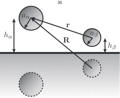
Particle-wall “self” mobility tensor (αα)
Particle-wall “pair” mobility tensor (αβ)
The high frequency dynamic viscosity of suspensions bound in channels and the distribution
The short-time self-diffusivity of a suspension bound by channel walls