On the Use of Conventional and Soft Computing Models for Prediction of Gross Calorific Value (GCV) of Coal

(1)

On the Use of Conventional and Soft Computing Models for Prediction of Gross Caloriﬁc Value (GCV) of Coal

Article in International Journal of Coal Preparation and Utilization · January 2011

DOI: 10.1080/19392699.2010.534683

CITATIONS

17

READS

18,364 2 authors:

Nazan Yalçın Erik Sivas Cumhuriyet University 105PUBLICATIONS 299CITATIONS

SEE PROFILE

Isik Yilmaz

Sivas Cumhuriyet University 194PUBLICATIONS 6,163CITATIONS

SEE PROFILE

All content following this page was uploaded by Nazan Yalçın Erik on 02 January 2014.

The user has requested enhancement of the downloaded file.

(2)

PLEASE SCROLL DOWN FOR ARTICLE

On: 24 January 2011

Access details: Access Details: [subscription number 772815469]

Publisher Taylor & Francis

Informa Ltd Registered in England and Wales Registered Number: 1072954 Registered office: Mortimer House, 37- 41 Mortimer Street, London W1T 3JH, UK

International Journal of Coal Preparation and Utilization

Publication details, including instructions for authors and subscription information:

http://www.informaworld.com/smpp/title~content=t713455898

On the Use of Conventional and Soft Computing Models for Prediction of Gross Calorific Value (GCV) of Coal

Nazan Yalçin Erk^a; Işk Yilmaz^a

a Faculty of Engineering, Department of Geological Engineering, Cumhuriyet University, Sivas, Turkey Online publication date: 22 January 2011

To cite this Article Erk, Nazan Yalçin and Yilmaz, Işk(2011) 'On the Use of Conventional and Soft Computing Models for Prediction of Gross Calorific Value (GCV) of Coal', International Journal of Coal Preparation and Utilization, 31: 1, 32 — 59

To link to this Article: DOI: 10.1080/19392699.2010.534683 URL: http://dx.doi.org/10.1080/19392699.2010.534683

Full terms and conditions of use: http://www.informaworld.com/terms-and-conditions-of-access.pdf This article may be used for research, teaching and private study purposes. Any substantial or systematic reproduction, re-distribution, re-selling, loan or sub-licensing, systematic supply or distribution in any form to anyone is expressly forbidden.

The publisher does not give any warranty express or implied or make any representation that the contents will be complete or accurate or up to date. The accuracy of any instructions, formulae and drug doses should be independently verified with primary sources. The publisher shall not be liable for any loss, actions, claims, proceedings, demand or costs or damages whatsoever or howsoever caused arising directly or indirectly in connection with or arising out of the use of this material.

(3)

ON THE USE OF CONVENTIONAL AND SOFT COMPUTING MODELS FOR PREDICTION OF GROSS CALORIFIC VALUE (GCV) OF COAL

NAZAN YALC¸ IN ERI˙K AND IS¸I˙K YILMAZ

Faculty of Engineering, Department of Geological Engineering, Cumhuriyet University, Sivas, Turkey

Gross calorific value (GCV) is an important characteristic of coal and organic shale; the determination of GCV, however, is difficult, time-consuming, and expensive and is also a destructive analysis.

In this article, the use of some soft computing techniques such as ANNs(artificial neural networks) andANFIS(adaptive neuro-fuzzy inference system) for predictingGCV(gross calorific value) of coals is described and compared with the traditional statistical model of MR (multiple regression). This article shows that the constructed ANFIS models exhibit high performance for predicting GCV. The use of soft computing techniques will provide new approaches and methodologies in prediction of some parameters in investigations about the fuel.

Keywords:ANFIS; ANN; Coal; Gross calorific value; Multiple regression; Soft computing

Received 12 July 2010; accepted 27 September 2010.

Authors are deeply grateful to the anonymous reviewers for their very constructive critics and suggestions that led to the improvement of the article.

Address correspondence to Is¸ik Yilmaz, Faculty of Engineering, Department of Geological Engineering, Cumhuriyet University, 58140 Sivas, Turkey. Tel.:þ90 346 219 1010 (1305 ext.); Fax: +þ90 346 219 1171; E-mail: iyilmaz@cumhuriyet.edu.tr

Copyright Taylor & Francis Group, LLC ISSN: 1939-2699 print=1939-2702 online DOI: 10.1080/19392699.2010.534683

Downloaded By: [yalcýn, nazan][TÜBTAK EKUAL] At: 07:41 24 January 2011

(4)

INTRODUCTION

Coal is valued for its energy content and, since the 1880s, is widely used to generate electricity. Steel and cement industries use coal as a fuel for extraction of iron from iron ore and for cement production. Coal mining is one of the most important mining activities in the world and there has been found very large terrestrial areas in different parts of the world [1, 2].

Turkey has also large coal reserves—about 9 gigatons (GT) [3]. The low-rank coals of Turkey represent the country’s major energy source with their relatively large geological reserves. The coal-bearing terrestrial tertiary deposits of Turkey overlie an area of approximately 110000 km², with the thicknesses of the coal seams varying between 0.05 and 87 m.

The country’s total coal reserves are 8–13 billion tons of low-quality coal and 1.3–4.0 billion tons of bituminous coal. Of the total annual lignite production of 90 million tons, 80%is consumed by thermal power plants.

The current total amount of coal consumption of the country, including imported coals as well, is about 60 megatons (MT) each year. Power plants and iron-steel plants consume most of this coal.

The coals in Turkey are generally low rank (lignite or sub-bituminous) formed in several different depositional environments at different geologic times and have differing chemical properties. The coal-bearing deposits, which have limnic characteristics, have relatively abundant reserves. Most of these coals have low calorific values, high-moisture, and high-ash contents.

Proximate and ultimate analyses characterize the chemical composition of coals. Proximate analyses include the determination of moisture content (TM), volatile matter (VM), ash (A), and fixed carbon (FC). While the ultimate analyses measure various element contents such as; carbon (C), hydrogen (H), nitrogen (N), sulfur (S), and oxygen (O). The ‘‘ultimate’’

analysis’’ gives the composition of the biomass in wt.%of carbon, hydrogen, and oxygen (the major components) as well as sulfur and nitrogen (if any).

The carbon determination includes that present in the organic coal substance and any originally present as mineral carbonate. The hydrogen determination includes that in the organic materials in coal and in all water associated with the coal. All nitrogen determined is assumed to be part of the organic materials in coal. The ‘‘proximate’’ analysis gives moisture content, volatile content, consisting of gases and vapors driven off during pyrol- ysis (when heated to 950C), the fixed carbon and the ash, the inorganic residue remaining after combustion in the sample, and the high heating

(5)

value (GCV) based on the complete combustion of the sample to carbon dioxide and liquid water. Proximate analysis is the most often used analysis for characterizing coals in connection with their utilization.

The calorific value is the measurement of heat or energy produced and is measured either as gross calorific value or net calorific value.

The difference being the latent heat of condensation of the water vapor produced during the combustion process. Gross calorific value (GCV) assumes all vapor produced during the combustion process is fully condensed. Net calorific value (NCV) assumes the water leaves with the combustion products without fully being condensed. Calorific value of coal can be determined by employing an apparatus called the Bomb Calorimeter. The amount of heat produced after 1 kg of a compound has undergone complete combustion (GCV). However, this instrument is expensive.

However, determination of gross calorific value (GCV) of a coal is time-consuming, expensive and involves destructive tests. If reliable predictive models could be obtained between GCV with quick, cheap, and nondestructive test results, it would be very valuable for characterization of coals.

Correlations have been a significant part of scientific research from the earliest days. In some cases, it is essential as it is difficult to measure the amount directly, and in other cases it is desirable, to ascertain the results with other tests through correlations. The correlations are generally semi-empirical based on some mechanics or purely empirical based on statistical analysis [4].

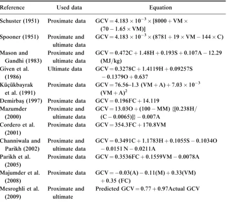
The calorific value is an essential measure of the quality coal burned at power plants; proximate and less common ultimate analyses are also used to evaluate the quality of thermal coal. The calorific value is usually expressed as the higher heating value or gross calorific value (GCV). Estimation of GCV from the elemental composition of fuel is one of the basic steps in performance modeling and calculations on combustion systems [5]. A number of equations have been developed for the prediction of gross calorific value (GCV) based on proximate and ultimate analysis by many authors such as Schuster [6], Spooner [7], Mazumder [8–9], Mason and Gandhi [10], Given et al. [11], Kucukbayrak et al. [12], Demirbas [13], Cordero et al.

[14], Channiwala and Parikh [5], Parikh et al. [15], Patel et al. [16], Majumder et al. [17], Mesroghli [18], etc., and a summary of the literature is given in Table 1.

(6)

Soft computing techniques such as fuzzy logic, artificial neural networks, genetic algorithms, neuro-fuzzy systems, etc. that were first used in the design of higher technology products are now being used in many branches of sciences and technologies, and their popularity is gradually increasing.

Earth sciences aim to describe very complex processes and need new technologies for data analyses. The number of studies in evolutionary algorithms and genetic programming, neural science and neural net systems, fuzzy set theory and fuzzy systems, fractal and chaos theory, and chaotic systems to solve problems in earth sciences (estimation of parameters; susceptibility, risk, vulnerability and hazard mapping;

interpretation of geophysical measurement results; many kinds of mining applications; etc.) have especially increased in the last five years.

Table 1.Summary of literature

Reference Used data Equation

Schuster (1951) Proximate data GCV¼4.18310³[8000þVM (701.65VM)]

Spooner (1951) Proximate and ultimate data

GCV¼4.18310³(8781þ19VM144C) Mason and

Gandhi (1983)

Proximate and ultimate data

GCV¼0.472Cþ1.48Hþ0.193Sþ0.107A12.29 (MJ=kg)

Given et al.

(1986)

Ultimate data GCV¼0.3278Cþ1.4119Hþ0.09257S 0.1379Oþ0.637

Ku¨c¸u¨kbayrak et al. (1991)

Proximate data GCV¼76.56–1.3 (VMþA)þ7.0310³ (VMþA)²

Demirbas¸(1997) Proximate data GCV¼0.196FCþ14.119 Mazumder

(2000)

GCV¼13.03Oþ(100MM) {[0.238H=

(C0.0065)]}0.007A Cordero et al.

(2001)

Proximate data GCV¼354.3FCþ170.8VM Channiwala and

Parikh (2002)

GCV¼0.3491Cþ1.1783Hþ0.1055S0.1034O 0.0151 N0.0211A

Parikh et al.

(2005)

Proximate data GCV¼0.3536FCþ0.1559VM0.0078A Majumder et al.

(2008)

Proximate data GCV¼ 0.03(A)0.11(M)þ0.33(VM) þ0.35 (FC)

Mesroghli et al.

(2009)

Proximate and ultimate

Predicted GCV¼0.77þ0.97Actual GCV

Note. Unit of GCV (calorific value) is MJ=kg; O: oxygen; C: carbon; S: sulfur; H:

hydrogen; A: ash; VM: volatile matter; FC: fixed carbon; MM: mineral matter; M: moisture.

(7)

The study presented herein aims to predict GCV of the coals from proximate and ultimate analyses results using a traditional statistical method (multiple regression [MR]) and two soft computing techniques (artificial neural networks [ANN] and adaptive neuro-fuzzy inference system [ANFIS]) and compares the models as to their prediction capabilities. A total of 74 coal samples were collected from various locations in Turkey and proximate and ultimate analyses performed. These parameters were correlated with the determined GCV first and statistically significant ones were selected. In order to establish predictive models, both statistical (multiple regression) and soft computing techniques (artificial neural networks and neuro-fuzzy models) were used and prediction performances were then analyzed.

TESTED COALS AND EXPERIMENTAL FRAMEWORK

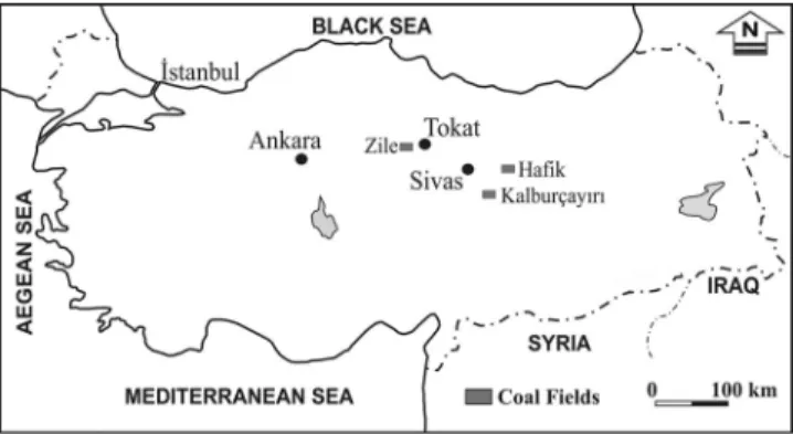
In this study, 74 samples were collected from the top to the base of the seams in three coal fields (Kalburc¸ayırı, Zile, Hafik) in Central Anatolia in Turkey (Figure 1). These samples were taken from along1 m lines using the channel-sampling technique, especially from the open-cast mine in the Kalburc¸ayırı and Zile fields and Hafik underground mine area. The sampling resolution for coal layers thicker than 20 cm was 10 cm; otherwise, it was equal to the thickness of the lithologically different layers.

The analyses (proximate and ultimate) were carried out according to American Society for Testing and Materials (ASTM) guidelines [19–23],

Figure 1. Location map of the sampling coal fields.

(8)

and they were converted into daf (dry ash free base) by calculation.

These analyses were performed in the Turkish General Directorate of Mineral Research and Exploration laboratory (MTA-MAT Laboratory, Ankara, Turkey) using standard analytical procedures. Coal-quality data (total moisture; ash; volatile matter; fixed carbon, calorific value; wt.%, daf) were obtained using an IKA 4000 adiabatic calorimeter; sulfur (wt.%, daf), carbon (wt.%, daf), hydrogen (wt.%, daf), and nitrogen (wt.%,daf) contents were determined using a LECO analyzer in the same laboratory.

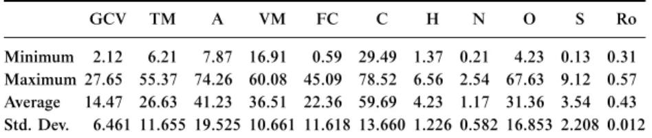
The coals tested in this study have reflectivity index (Ro) between 0.31–0.57 with an average value of 0.43, and they were categorized as

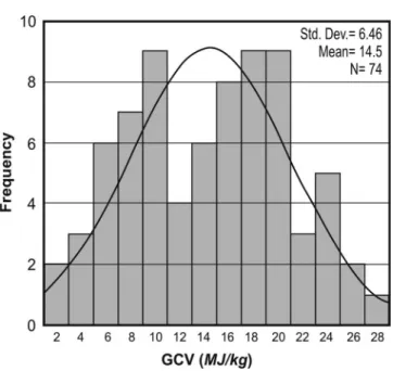
‘‘sub-bituminous=low-rank B=C coal.’’ The gross calorific value of the coals ranged between 2.12 and 27.65 MJ=kg with an average value of 14.47 MJ=

kg. The results and their basic test statistics are tabulated in Table 2.

DATA PROCESSING

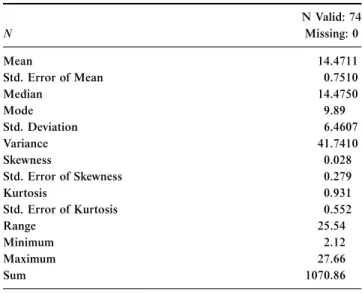
Particular attention is required to select the data set having a normal distribution. In order to characterize the variation of GCV used as an independent value, descriptive statistics such as minimum, maximum, mean, mode, median, variance, standard deviation, skewness, and kurtosis were calculated using the SPSS Version 10.0 [24] package. Table 3 shows that the independent values show almost normal distribution.

However, it is close to the normal distribution and data are skewed right and showed a kurtosis (Figure 2). It can be seen that the respective skewness and kurtosis values of 0.028 and 0.931 were very low. In conclusion, it was evident that the regression analyses will work well in this case.

In order to establish the predictive models among the parameters obtained in this study, simple regression analysis were performed in

Table 2.Basic statistics of the results obtained from analyses

GCV TM A VM FC C H N O S Ro

Minimum 2.12 6.21 7.87 16.91 0.59 29.49 1.37 0.21 4.23 0.13 0.31 Maximum 27.65 55.37 74.26 60.08 45.09 78.52 6.56 2.54 67.63 9.12 0.57 Average 14.47 26.63 41.23 36.51 22.36 59.69 4.23 1.17 31.36 3.54 0.43 Std. Dev. 6.461 11.655 19.525 10.661 11.618 13.660 1.226 0.582 16.853 2.208 0.012

Note.Unit of GCV is MJ=kg, others are%. Ro is the reflectivity index.

(9)

Figure 2. Frequency distribution of GCV values of samples used in analyses.

Table 3.Descriptive statistics for GCV as an independent value N Valid: 74

N Missing: 0

Mean 14.4711

Std. Error of Mean 0.7510

Median 14.4750

Mode 9.89

Std. Deviation 6.4607

Variance 41.7410

Skewness 0.028

Std. Error of Skewness 0.279

Kurtosis 0.931

Std. Error of Kurtosis 0.552

Range 25.54

Minimum 2.12

Maximum 27.66

Sum 1070.86

(10)

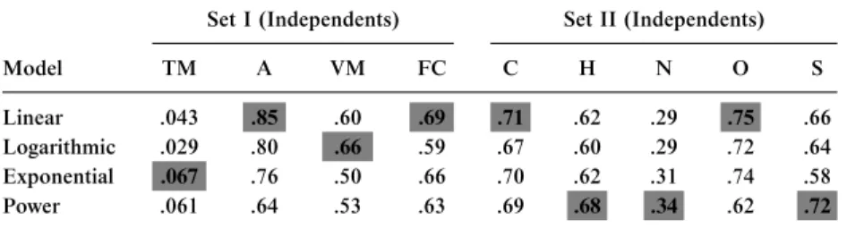
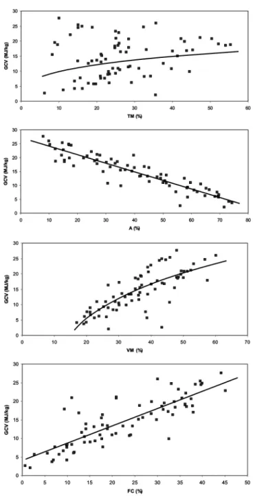
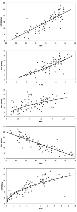
the first stage of the analysis. The relations between GCV with other parameters were analyzed employing linear, power, logarithmic, and exponential functions. Statistically significant and strong correlations were then selected (Table 4), and regression equations were established among GCV with proximate (Set I) and ultimate (Set II) analyses results (Table 5). All obtained relationships were found to be statistically significant according to the Student’sttest with 95%confidence, except nitrogen (N). Figures 3 and 4 show the plot of the GCV versus moisture content (TM), ash (A), volatile matter (VM), fixed carbon (FC), carbon (C), hydrogen (H), nitrogen (N), sulfur (S), and oxygen (O).

MULTIPLE REGRESSION MODELS

Multiple regression is employed to account for (predict) the variance in an interval dependent, is based on linear combinations of interval, dichotomous, or dummy independent variables. The general purpose

Table 4. Correlation coefficients (R²) obtained from the simple regressions between GCV with other parameters

Set I (Independents) Set II (Independents)

Model TM A VM FC C H N O S

Linear .043 .85 .60 .69 .71 .62 .29 .75 .66

Logarithmic .029 .80 .66 .59 .67 .60 .29 .72 .64

Exponential .067 .76 .50 .66 .70 .62 .31 .74 .58

Power .061 .64 .53 .63 .69 .68 .34 .62 .72

Note. Gray-filled cells show the highest correlation coefficients (R²); gray-filled cells with borders show strong correlations that were included in the models.

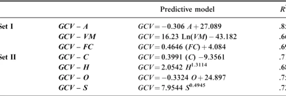
Table 5.Predictive models for assessment of GCV

Predictive model R²

Set I GCV – A GCV¼ 0.306Aþ27.089 .85

GCV – VM GCV¼16.23 Ln(VM)43.182 .66 GCV – FC GCV¼0.4646 (FC)þ4.084 .69

Set II GCV – C GCV¼0.3991 (C)9.3561 .71

GCV – H GCV¼2.0542H^1.3114 .68

GCV – O GCV¼ 0.3324Oþ24.897 .75

GCV – S GCV¼7.9544S^0.4945 .72

(11)

Figure 3. GCV versus moisture content (TM), ash (A), volatile matter (VM), and fixed carbon (FC) graphs for Set I.

(12)

Figure 4. GCV versus carbon (C), hydrogen (H), nitrogen (N), oxygen (O), and sulfur (S) graphs for Set II.

(13)

of multiple regression is to learn more about the relationship between several independent or predictor variables and a dependent or criterion variable. The multiple regression equation takes the form y¼b1x1þ b2x2þ þbnxnþc. The b’s are the regression coefficients, representing the amount the dependent variable y changes when the corresponding independent changes one unit. The c is the constant, where the regression line intercepts the y-axis, representing the amount the dependent y will be when all the independent variables are 0. The standardized versions of the b coefficients are the beta weights, and the ratio of the beta coefficients is the ratio of the relative predictive power of the independent variables. Associated with multiple regression is R², a coefficient of multiple determination, which is the amount of variance in the dependent variable explained collectively by all of the independent variables. The major conceptual limitation of all regression techniques is that one can only ascertain relationshipsbut can never be sure about the underlyingcausalmechanism [25].

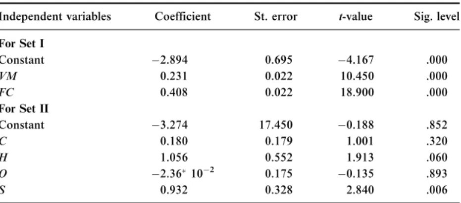
Two multiple regression analyses carried out to correlate the measured GCV to two selected data sets, namely, Set I (volatile matter, fixed carbon) and Set II (carbon, hydrogen, nitrogen, sulfur, oxygen) revealed the following results. In the multiple regression analyses of Set I, ‘‘Ash’’

was an excluded variable because of colinearity. Predictors in this model were constant, fixed carbon (FC) and volatile matter (VM), and the dependent variable was GCV. Model summaries of multiple regression analyses for prediction ofGCVcan be seen in Table 6:

Table 6.Model summaries of multiple regressions for prediction of GCV

Independent variables Coefficient St. error t-value Sig. level For Set I

Constant 2.894 0.695 4.167 .000

VM 0.231 0.022 10.450 .000

FC 0.408 0.022 18.900 .000

For Set II

Constant 3.274 17.450 0.188 .852

C 0.180 0.179 1.001 .320

H 1.056 0.552 1.913 .060

O 2.3610² 0.175 0.135 .893

S 0.932 0.328 2.840 .006

Ais excluded because of colinearity.

(14)

Figure 5. Cross-correlation of predicted and observed values of GCV for multiple regression model.

(15)

GCV ¼0:231VMþ0:408FC2:894; ð1Þ GCV ¼0:180Cþ1:056H2:3610²Oþ0:932S3:274: ð2Þ In fact, the coefficient of determination between the measured and predicted values is a good indicator to check the prediction performance of the model. Figure 5 shows the relationships between measured and predicted values obtained from the models forGCV, with good coefficients of multiple determination. In this study, variance accounts for (VAF;

Equation 3) and root mean square error (RMSE; Equation 4) indices were also calculated to control the performance of the prediction capacity of predictive models developed in the study as employed by Alvarez and Babuska [26], Finol et al. [27], Yilmaz and Yu¨ksek [25, 28]:

VAF ¼ 1varðyy⁰Þ varðyÞ

100; ð3Þ

RMSE¼

ffiffiffiffiffiffiffiffiffiffiffiffiffiffiffiffiffiffiffiffiffiffiffiffiffiffiffiffiffiffi 1

N X^N

i¼1

ðyy⁰Þ² vu

ut ; ð4Þ

whereyandy⁰ are the measured and predicted values, respectively. The calculated indices are given in Table 6. If the VAF is 100 and RMSE is 0, then the model will be excellent. The obtained values of VAF and RMSE given in Table 7 indicate the higher prediction performances.

Table 7.Performance indices (RMSE, VAF, andR²) for models used

Model RMSE VAF (%) (R²)

Multiple Regression

Set I 1.645 93.125 .934

Set II 2.966 71.819 .782

Artificial Neural Networks

Set I 1.019 97.767 .981

Set II 1.341 96.584 .966

Adaptive Neuro-Fuzzy Inference System

Set I 0.565 99.383 .994

Set II 0.717 99.053 .989

Note.RMSE¼root mean square error; VAF¼value account for.

(16)

ARTIFICIAL NEURAL NETWORK (ANN) MODELS

When the materials are natural materials, many uncertainties will be in question and material will never be known with certainty. That’s why some methodologies in artificial neural networks, fuzzy systems, and evolutionary computation have been successfully combined, and new techniques called soft computing or computational intelligence have been developed in recent years. These techniques are attracting more and more attention in several research fields because they tolerate a wide range of uncertainty [29]. Artificial neural networks are data-processing systems devised via imitating brain activity and have performance characteristics like biological neural networks. ANN has a lot of important capabilities such as learning from data, generalization, working with unlimited number of variables [30]. Neural networks may be used as a direct substitute for auto correlation, multivariable regression, linear regression, trigonometric, and other statistical analysis techniques [31].

Neural networks, with their remarkable ability to derive meaning from complicated or imprecise data, can be used to extract patterns and detect trends that are too complex to be noticed by either humans or other computer techniques. Rumelhart and McClelland [32] reported that the main characteristics of ANN include large-scale parallel distributed processing, continuous nonlinear dynamics, collective computation, high fault-tolerance, self-organization, self-learning, and real-time treatment.

A trained neural network can be thought of as an ‘‘expert’’ in the cate- gory of information it has been given to analyze. This expert can then be used to provide projections given new situations of interest and answer ‘‘what if ’’ questions.

When a data stream is analyzed using a neural network, it is possible to detect important predictive patterns that are not previously apparent to a nonexpert. Thus, the neural network can act as an expert. The particular network can be defined using three fundamental components:

transfer function, network architecture, and learning law [33]. It is essential to define these components, to solve the problem satisfactorily.

Neural networks consist of a large class of different architectures, and there are many kinds of ANN models, among which the back propagation (BP) model is the most widely used, and it is an instructive training model. The basic idea of the back propagation learning algorithm [34] is the repeated application of the chain rule to compute the influence of each weight in the network with respect to arbitrary error function E:

(17)

@E

@v_ij¼@E

@Y_i

@Yi

@net_i

@neti

@v_ij ; ð5Þ

wherevijis the weight from neuronjto neuroni, Yiis the output, andneti

is the weighted sum of the inputs of neuroni.

Once the partial derivative for each weight is known, the aim of minimizing the error function is achieved by performing a simple gradient descent:

v_ijðtþ1Þ ¼v_ijðtÞ r@E

@v_ijðtÞ; ð6Þ

wheret denotes time,r is the learning parameter.

It is accepted that the most useful neural networks in prediction and decision algorithms are back propagation and Radial Basis Function (RBF) networks. In this article, back propagation algorithm, created by generalizing the Widrow–Hoff learning rule to multiple-layer networks and nonlinear differentiable transfer functions, is used. A back propagation consists of an input layer, several hidden layers, and output layers. All of those layers may contain multiple nodes [35].

The inputsxn, n¼1,. . ., n to the neuron are multiplied by weightswni

and summed up together with the constant bias termQi. The resultingxi

is the input to the activation functiony. The activation function was originally chosen to be a relay function, but for mathematical convenience a hyperbolic tangent (tanh) or a sigmoid function are most commonly used. Hyperbolic tangent is defined as

fðxÞ ¼tanhðxÞ ¼e^xe^x

e^xþe^x: ð7Þ

The output of nodeibecome

yi¼f X^k

j¼1

wikxjþQi

!

: ð8Þ

Connecting several nodes in parallel and series, a multi layer percep- tion (MLP) network is formed. The following equations explain mathematical notation of back propagation algorithm.

a^m_0:j¼ ðx_mÞ_j¼x^m_j ; ð9Þ

(18)

c^m_i:j ¼X^sⁱ¹

k¼1

w_i:j;ka^m_i1:kþb_i:j; i>0; ð10Þ

a^m_i:j ¼Fi:jðc^m_i:jÞ; i>0: ð11Þ

a^m_i:j¼F_i:j X^sⁱ¹

k¼1

w_i:j;ka^m_i1:kþb_i:j

!

ð12Þ

a^m_L:1 ¼ym ð13Þ

1

2 y_mt_m

²¼1

2ðymtmÞ²¼e²_m¼em ð14Þ Learning procedure can be given as follows:

1. Selection of random and small-sized (between 0–1) numbers for all weight and bias.

2. Calculation of network output and comparison with the destination output.

3. If the network output is approximately equal to the desired output, then continue with step 1, and, if not, weights are corrected according to the correction rule and then continue with step 1.

All data were first normalized and divided into three data sets such as training (1=2 of all data), test (1=4 of all data), and verification (1=4 of all data). In this study MatLab 7.1 [36] software was used in neural network analyses having a three-layer feed-forward network in both of the two sets. They consist of an input layer (three neurons in Set I, four neurons in Set II), one hidden layer (seven neurons in Set I, nine neurons in Set II) and one output layer (Figure 6). In the analyses, learning and momentum parameters, networks training, and activation (transfer) function for all layers were respectively adjusted to 0.01, 0.9, trainLm, and tansig. As in many other network training methods, models and parameters were used to be able to reach minimum RMS values, and the network goal was reached at the end of 421 and 537 iterations in models of Set I and Set II, respectively.

Cross-correlation between predicted and observed values (Figure 7) indicated that the ANN model constructed is highly acceptable for prediction ofGCV. RMSE, VAF, andR²values are tabulated in Table 7.

(19)

ADAPTIVE NEURO-FUZZY INFERENCE SYSTEM (ANFIS) MODELS

In ANFIS, both of the learning capabilities of a neural network and reasoning capabilities of fuzzy logic were combined in order to give enhanced prediction capabilities, as compared to using a single method- ology alone. The goal of ANFIS is to find amodelor mappingthat will correctly associate the inputs (initial values) with the target (predicted values). The fuzzy inference system (FIS) is a knowledge representation where each fuzzy rule describes a local behavior of the system. The network structure that implements FIS and employs hybrid-learning rules for training is called ANFIS.

LetXbe a space of objects andxbe a generic element ofX. A classical setAXis defined as a collection of elements or objectsx2Xsuch that eachxcan either belong or not belong to the setA. By defining acharac- teristic functionfor each elementxinX, we can represent a classical setA by a set of ordered pairs (x, 0) or (x, 1) that indicatesx=62Aorx 2A, respectively. On the other hand, a fuzzy set expresses the degree to which

Figure 6. Neural network structure used in the study.

(20)

Figure 7. Cross-correlation of predicted and observed values of GCV for ANN model.

(21)

an element belongs to a set. Hence, thecharacteristic functionof a fuzzy set is allowed to have values between 0 and 1, which denotes the degree of membership of an element in a given set. So a fuzzy setAinXis defined as a set of ordered pairs:

A¼ f½x;lAðxÞjx2Xg; ð15Þ wherelA(x) is called themembership function(MF) for the fuzzy setA.

The MF maps each element ofXto a membership grade (or a value) between 0 and 1. UsuallyXis referred to as theuniverse of discourseor simply the universe. The most widely used MF is the generalized bell MF (or the bell MF) for data having normal-like distribution, which is specified by three parameters {a, b, c} and defined as [37]:

bellðx;a;b;cÞ ¼1=ð1þ jx ðc=aÞj^2bÞ: ð16Þ Parameterbis usually positive. A desired bell MF can be obtained by a proper selection of the parameter set {a, b, c}. During the learning phase of ANFIS, these parameters are changing continuously in order to minimize the error function between the target output values and the calculated ones [38, 39].

The proposed neuro-fuzzy model of ANFIS is a multilayer neural network-based fuzzy system. Its topology is shown in Figure 8, and the system has a total of five layers. In this connected structure, the input and output nodes respectively represent the training values and the predicted values; there are nodes functioning as membership functions (MFs) and rules and in the hidden layers. This architecture has the benefit that it eliminates the disadvantage of a normal feed forward multilayer network, where it is difficult for an observer to understand or modify the network.

For simplicity, we assume that the examined fuzzy inference system has two inputs xand y and one output. For a first-order Sugeno fuzzy model, a common rule set with two fuzzy if-then rules is defined as

Rule 1:If xis A₁ andyisB₁;thenf₁¼p₁xþq₁yþr₁; ð17Þ

Rule 2:If xis A₂ andyisB₂;thenf₂¼p₂xþq₂yþr₂: ð18Þ

(22)

As seen from Figure 8b, different layers of ANFIS have different nodes. Each node in a layer is either fixed or adaptive [40]. Different layers with their associated nodes are described below:

1. Layer 1. Every nodeIin this layer is an adaptive node. Parameters in this layer are calledpremise parameters.

2. Layer 2. Every node in this layer is a fixed node labeledP, whose output is the product of all the incoming signals. Each node output represents the firing strength of a rule.

3. Layer 3. Every node in this layer is a fixed node labeled N. Theith node calculates the ratio of theith rules’ firing strength. Thus the outputs of this layer are callednormalized firing strengths.

4. Layer 4. Every nodeiin this layer is an adaptive node. Parameters in this layer are referred to asconsequent parameters.

Figure 8. Type-3 fuzzy reasoning (a) and equivalent ANFIS (b).

(23)

5. Layer 5. The single node in this layer is a fixed node labeledR, which computes the overall output as the summation of all incoming signals.

The learning algorithm for ANFIS is a hybrid algorithm, which is a combination of gradient descent and the least-squares method. More specifically, in the forward pass of the hybrid-learning algorithm, node outputs go forward until layer 4 and the consequent parameters are ident- ified by the least-squares method [40]. In the backward pass, the error signals propagate backwards and the premise parameters are updated by gradient descent. Table 8 summarizes the activities in each pass.

The consequent parameters are optimized under the condition that the premise parameters are fixed. The main benefit of the hybrid approach is that it converges much faster since it reduces the search space dimensions of the original pure back propagation method used in neural networks. The overall output can be expressed as a linear combination of the consequent parameters. The error measure to train the above-mentioned ANFIS is defined as [41]:

E ¼ Xⁿ

k¼1

ðfkf_k⁰Þ²; ð19Þ

wherefkandf⁰kare thekth desired and estimated output, respectively, and nis the total number of pairs (inputs-outputs) of data in the training set.

In this study, a hybrid intelligent system called ANFIS (the adaptive neuro-fuzzy inference system) for predicting GCV was also applied.

ANFIS was trained with the help of Matlab version 7.1 [36]; the SPSS 10.0 [24] package was used for RMSE and statistical calculations. Bell function was used as MF type, and output MF was linear.

According to the RMSE, VAF, R² values (Table 7) and cross- correlation between predicted and observed values (Figure 9), the ANFIS model constructed to predict GCV has a very high prediction performance.

Table 8.Forward and backward pass for ANFIS

Forward pass Backward pass Premise parameters Fixed Gradient descent Consequent parameters Least-squares estimator Fixed

Signals Node outputs Error signals

(24)

Figure 9. Cross-correlation of predicted and observed values of GCV for ANFIS model.

(25)

RESULTS AND CONCLUSIONS

In this article, use of multiple regression (MR), artificial neural network (ANN), and artificial neuro-fuzzy inference system (ANFIS) models for prediction of gross calorific value of coals was described and compared.

It appears that there is a possibility of estimating GCV of coals by using the proposed empirical relationships and soft computing models.

According to the results of simple regression analyses, there are statistically meaningful relationships between gross calorific value with ash, volatile matter, fixed carbon, carbon, hydrogen, sulfur, and oxygen. The models of multiple regression, artificial neural network, artificial neuro-fuzzy inference system for the prediction of the gross calorific value were then constructed using three inputs for Set I (ash, volatile matter, fixed carbon) and four inputs for Set II (carbon, hydrogen, sulfur, oxygen) and one output (GCV).

The results of the present article and their conclusions can be drawn as follows:

1. The results of the models for prediction of the gross calorific value showed that the equations obtained from the multiple regression models have high-prediction performances.

2. In order to predict the gross calorific value, ANN models having three (for Set I) and four (for Set II) inputs, with one output was applied successfully and exhibited more reliable predictions than the regression models.

3. The ANFIS model for prediction of gross calorific value revealed the most reliable predictions when compared with the multiple regression and ANN models.

The comparison of VAF, RMSE indices, and coefficient of multiple determination (R²) for predicting GCV revealed that prediction performances of the artificial neuro-fuzzy inference system model are higher than those of multiple regression equations and artificial neural networks (Figure 10). In order to show the deviations from the observed values of GCV, the distances of the predicted values from the models constructed from the observed values were also calculated and graphics were drawn (Figure 11). These graphics indicated that the deviation intervals (in Set I: 1.00–þ1.65; in Set II: 2.21–þ2.34) of the predicted values from ANFIS are smaller than the deviation intervals of ANN (in

(26)

Set I:3.60–þ2.49; in Set II: -3.16–þ4.13) and multiple regression (in Set I:6.56–þ3.72; in Set II: -9.67–þ8.20).

It is shown that the constructed ANN and ANFIS models exhibit higher performance than multiple regression models for predicting

Figure 10. Comparison graphics of RMSE, VAF, and R² for the models (MR, ANN, ANFIS).

(27)

GCV. As is known, the potential benefits of soft computing models extend beyond the high computation rates. Higher performances of the soft computing models were sourced from greater degree of robustness and fault tolerance than traditional statistical models because there are many more processing neurons, each with primarily local connections.

Patel et al. [16] had estimated gross calorific value using ANN model and obtained high model performance; however, Mesroghli et al. [18]

had reported that ANNs were not better or much different from a regression model.

The performance comparison also showed that the soft computing techniques are good tools for minimizing the uncertainties, and their use will also provide new approaches and methodologies and minimize the potential inconsistency of correlations. The results of this article will provide dissemination of important results of the use of soft computing

Figure 11. Graphics showing the variation of the values predicted by MR, ANN, and ANFIS models from the observed values.

(28)

technologies in fuel sciences and will serve as an example for fuel scientists and engineers engaged in this area of interest.

REFERENCES

1. Marschalko, M., M. Fuka, and L. Treslin. 2008. Influence of mining activity on selected landslide in the Ostrava-Karvina coalfield. ACTA Montanistica Slovaca13: 58–65.

2. Marschalko, M., and L. Treslin. 2009. Impact of underground mining to slope deformation genesis at Doubrava Ujala. ACTA Montanistica Slovaca 14: 232–240.

3. Turkish Lignite Authority (TKI). 2008. Available at http://www.tki.gov.tr (in Turkish).

4. Yilmaz, I. 2006. Indirect estimation of the swelling percent and a new classi- fication of soils depending on liquid limit and cation exchange capacity.

Engineering Geology85: 295–301.

5. Channiwala, S. A., and P. P. Parikh. 2002. A unified correlation for estimating HHV of solid, liquid and gaseous fuels.Fuel81: 1051–1063.

6. Schuster, V. F. 1951. U¨ ber die berechnung des heizwertes von kohlen aus der immediatzusammensetzung.Brennstoff – Chemie32: 19–20.

7. Spooner, C. E. 1951. Swelling power of coal.Fuel30: 193–202.

8. Mazumder, B. K. 1954. Coal systematics: deductions from proximate analysis of coal. part I.Journal of Scientific and Industrial Research13B: 857–863.

9. Mazumder, B. K. 2000. Theoretical oxygen requirement for coal combustion:

Relationship with its calorific value.Fuel79: 1413–1419.

10. Mason, D. M., and K. N. Gandhi. 1983. Formulas for calculating the calorific value of coal and chars.Fuel Processing Technology7: 11–22.

11. Given, P. H., D. Weldon, and J. H. Zoeller. 1986. Calculation of calorific values of coals from ultimate analyses: Theoretical basis and geochemical implications.Fuel65: 849–854.

12. Kucukbayrak, S., B. Durus, A. E. Mericboyu, and E. Kadioglu. 1991.

Estimation of calorific values of Turkish lignites.Fuel70: 979–981.

13. Demirbas, A. 1997. Calculation of higher heating values of biomass fuels.

Fuel76: 431–434.

14. Cordero, T., F. Marquez, J. Rodriquez-Mirasol, and J. J. Rodriguez. 2001.

Predicting heating values of lignocellulosic and carbonaceous materials from proximate Analysis.Fuel80: 1567–1571.

15. Parikh, J., S. A. Channiwala, and G. K. Ghosal. 2005. A correlation for calculating HHV from proximate analysis of solid fuels.Fuel84: 487–494.

16. Patel, S. U., B. J. Kumar, Y. P. Badhe, B. K. Sharma, S. Saha, S. Biswas, A. Chaudhury, S. S. Tambe, and B. D. Kulkarni. 2007. Estimation of gross calorific value of coals using artificial neural networks.Fuel86: 334–344.

(29)

17. Majumder, A. K., R. Jain, J. P. Banerjee, and J. P. Barnwal. 2008. Develop- ment of a new proximate analysis based correlation to predict calorific value of coal.Fuel87: 3077–3081.

18. Mesroghli, S. H., E. Jorjani, and S. C. Chelgani. 2009. Estimation of gross calorific value based on coal analysis using regression and artificial neural networks.International Journal of Coal Geology79: 49–54.

19. American Society for Testing and Materials (ASTM). 2004. D5307-97, Stan- dard Test Method for Determination of Boiling Range Distribution of Crude Petroleum by Gas Chromatography. In 2004 Annual Book of ASTM Stan- dards, Gaseous Fuels; Coal and Coke, Vol. 05.06. Philadelphia, PA: ASTM.

20. American Society for Testing and Materials (ASTM). 2004. D3174, Stan- dard Method for Ash in the Analysis Sample of Coal and Coke from Coal.

In 2004 Annual Book of ASTM Standards, Gaseous Fuels; Coal and Coke, Vol. 05.06. Philadelphia, PA: ASTM.

21. American Society for Testing and Materials (ASTM). 2004. D3175, Stan- dard Method for Volatile Matter in the Analysis Sample of Coal and Coke.

In 2004 Annual Book of ASTM Standards, Gaseous Fuels; Coal and Coke, Vol. 05.06. Philadelphia, PA: ASTM.

22. American Society for Testing and Materials (ASTM). 2004. D3302, Stan- dard Method for Total Moisture in Coal, in 2004 Annual Book of ASTM Standards, Gaseous Fuels: Coal and Coke, Vol. 05.06. Philadelphia, PA:

ASTM.

23. American Society for Testing and Materials (ASTM). 2004. D5373, Stan- dard Test Methods for Instrumental Determination of Carbon, Hydrogen and Nitrogen in Laboratory Samples of Coal and Coke, in2004 Annual Book of ASTM Standards, Gaseous Fuels: Coal and Coke, Vol. 05.06. Philadelphia, PA: ASTM.

24. SPSS 10.0.1. 1999. Statistical Analysis Software (Standard Version).

Chicago, IL: SPSS Inc.

25. Yilmaz, I., and A. G. Yu¨ksek. 2009. Prediction of the strength and elasticity modulus of gypsum using multiple regression, ANN, ANFIS models and their comparison. International Journal of Rock Mechanics and Mining Sciences46: 803–810.

26. Alvarez, G. M., and R. Babuska. 1999. Fuzzy model for the prediction of unconfined compressive strength of rock samples. International Journal of Rock Mechanics and Mining Sciences36: 339–349.

27. Finol, J., Y. K. Guo, and X. D. Jing. 2001. A rule based fuzzy model for the prediction of petrophysical rock parameters. Journal of Petroleum Science Engineering29: 97–113.

28. Yilmaz, I., and A. G. Yu¨ksek. 2008. An example of artificial neural network application for indirect estimation of rock parameters.Rock Mechanics and Rock Engineering41: 781–795.

(30)

29. Jin, Y., and J. Jiang. 1999. Techniques in neural-network based fuzzy system identification and their application to control of complex systems. InFuzzy Theory Systems, Techniques and Applications, ed. C. T. Leondes. New York:

Academic Press.

30. Kaynar, O., I. Yilmaz, and F. Demirkoparan. 2011. Forecasting of natural gas consumption with neural network and neuro fuzzy system.Energy Edu- cation Science & Technology Part A: Energy Science and Research26: 221–238.

31. Singh, T. N., R. Kanchan, A. K. Verma, and S. Singh. 2003. An intelligent approach for prediction of triaxial properties using unconfined uniaxial strength.Mining Engineering Journal5: 12–16.

32. Rumelhart, D., and J. McClelland. 1986. Parallel Distributed Processing:

Explorations in the Microstructure of Cognition. Cambridge, MA: MIT Press.

33. Simpson, P. K. 1990.Artificial Neural System-Foundation, Paradigm, Appli- cation and Implementation. New York: Pergamon Press.

34. Rumelhart, D. D., G. E. Hinton, and R. J. Williams. 1986. Learning internal representations by error propagation. In Parallel Distributed Processing:

Explorations in the Microstructure of Cognition, Vol. 1, eds. D. E. Rumelhart and J. McClelland. Cambridge, MA: MIT Press.

35. Yilmaz, I. 2009. Landslide susceptibility mapping using frequency ratio, logistic regression, artificial neural networks and their comparison: A case study from Kat landslides (Tokat-Turkey). Computer and Geosciences 35:

1125–1138.

36. Matlab 7.1. 2005.Software for Technical Computing and Model-Based Design.

Natick, MA: MathWorks, Inc.

37. Jang, J. S. R., and S. Chuen-Tsai. 1995. Neuro-fuzzy modeling and control.

Proc. IEEE83: 378–406.

38. Lee, C. C. 1990. Fuzzy logic in control systems: Fuzzy logic controller. I IEEE Transactions on Systems, Man, and Cybernetics20: 404–418.

39. Lee, C. C. 1990. Fuzzy logic in control systems: Fuzzy logic controller.II IEEE Transactions on Systems, Man, and Cybernetics20: 419–435.

40. Jang, J. R. 1993. ANFIS: Adaptive-network-based fuzzy inference system.

IEEE Transactions on Systems, Man, and Cybernetics23: 665–685.

41. Loukas, Y. L. 2001. Adaptive neuro-fuzzy inference system: An instant and architecture-free predictor for improved QSAR studies.Journal of Medical Chemistry44: 2772–2783.

View publication stats