These discrepancies motivate models of dark matter with properties that differ significantly from the standard paradigm. The modification of ΛCDM to include self-interacting dark matter (SIDM), sometimes called the ΛSIDM model, is.
Introduction
The General Picture: Evolving Dark Matter in the Early Universe
The Boltzmann Equation
Assume that dark matterψ is a stable particle that annihilates with the thermal annihilation cross section hσvi. Generalizing the traditional treatment, we allow for the possibility that the dark matter mass ˜mψ(φ) is a function of a real scalar chameleon fieldφ, and denote the φ-dependent masses and couplings with a tilde.
Gauged Dark Matter
A Toy Model for Varying Coupling
Having generalized the usual treatment of dark matter as a fluid to the case where there is a chameleon field that determines the properties of dark matter, we now turn to specific examples of particle physics models where these phenomena can arise. If we can neglect factors of (∂µf /˜ f˜ ) compared to all other mass scales in the theory (except the Planck mass), then the Lagrangian simplifies to the approximate gauge-invariant form.
The Cosmological Equations of Motion
Thus, the term proportional to ˜f0/f˜ should be small compared to the term containing ˜m0/m, given that ˜˜ f0/f˜∼m˜0/m˜ to within a few orders of magnitude lies – a condition we will enforce later. We calculate the energy momentum tensor forψ by varying the action with respect to the metric.
Chameleon Behavior
Exponential Potentials
With these comments in mind, we therefore choose the form the effective potential and U(1) coupling should be. We therefore require m2, m3mψ to suppress higher-dimensional operators involving derivatives of ˜mψ and ˜f when expanding the action.
An Attractor Solution
Similarly, if (1.46) holds during matter dominance, when. then we can simply determine φ0, the value of φtoday, which is needed to calculate the values of today's φ-dependent parameters. 1.49). It follows that HR decreases faster than ˜mφ,ph over time, while during matter dominance HM and ˜mφ,ph have the same dependence.
Particle Physics Interactions and Constraints
- Breaking the Dark U(1) Symmetry
- The Dark Matter Annihilation Cross Section
- Corrections to the Cross Section
- The Annihilation Cross Section
- The Scattering Cross Section
- Dark Decays
We assume that the dark matter is the heaviest particle in the dark sector, so that ˜mψ. Note, however, that if thermal averaging is necessary (according to [38]), we must use the dark sector temperatureTd in the expression.
Numerical Solutions
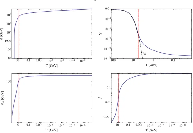
The top right panel shows the annihilation cross section σv versus the scattering cross section σ/m˜ψ, both estimated at x0 today. The scattering cross-section rapidly approaches its asymptotic value by the time of the dark matter freeze-out, while the annihilation cross-section is still growing by orders of magnitude from the freeze-out until now.

Conclusions
However, in the case of the Euclidean vacuum we have both the reduced density matrix ρN and the full quantum state |Ωi. Moch, “The Top Quark and Higgs Boson Masses and the Stability of the Electroweak Vacuum,” Phys.
Introduction
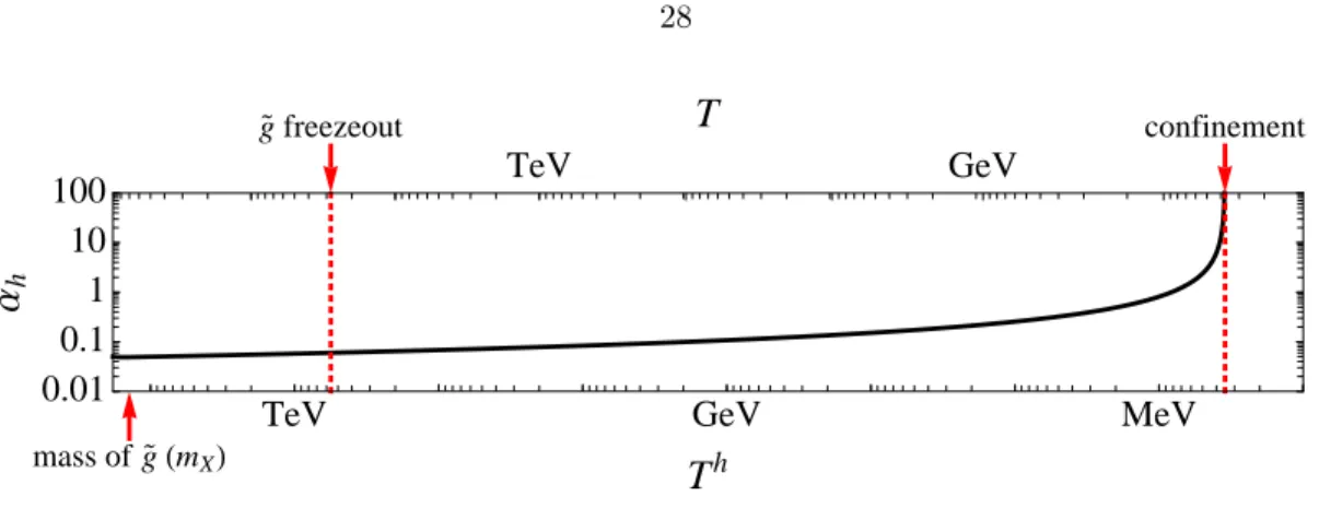
In this model, the dark matter is a ~10 TeV hidden gluino which freezes out in the early universe. In the second case, the hidden sector is connected to the visible sector through connecting fields.
Astrophysical Evidence for Self-Interacting Dark Matter
In §2.3, we start with the simplest possible case: non-supersymmetric pure hidden sectors and glueball dark matter. We then move on to supersymmetric models with pure hidden sectors and glueball dark matter.
Glueball Dark Matter
- Glueball Self-Interactions
- Glueball Relic Density
- Viable Glueball Parameters
The self-interaction cross section and the relic density are given in the (ξΛ,Λ) plane, where Λ is the confinement scale in the hidden sector and ξΛ ≡ Th/T is the ratio of hidden to visible sector temperatures at the time Th = Λ. The self-interaction cross section is in the range hσTi/mX = 0.1–1 cm2/g in the shaded region.
Glueballino Self-Interactions
The inelastic effects are not modeled in the ΛSIDM simulations and are therefore not well understood. 10 cm2/g with mX &TeV, the parameters must be in the classical scattering regime, mXv Λ. Scattering by Yukawa potentials has been studied in this regime in the context of classical complex plasmas and simple analytical fits to numerical results for the transfer cross section have been derived.
The transfer cross section decreases as a function of in the classical regime; thus systems with large characteristic velocities have smaller diameters, everything else looked different.
Glueballino Relic Density
- Gluino Freezeout
- The WIMPless Miracle and AMSB
As we will see, for most of the parameter space of interest, gluinos freeze at visible sector temperatures at or above TSM ≈ 300 GeV, so that all SM particles are relativistic andg∗S =g∗ = 106.75. Although there may be Minimum Supersymmetric Standard Standard (MSSM) superpartners with masses low enough to contribute tog∗ to the freeze, we assume that the contribution is negligible, with most of the visible spectrum of the supersymmetric partner being above mX. For weakly scaled masses and weakly interacting coupling forces, ΩX is of the desired magnitude; this coincidence is the essence of the WIMP miracle.
In each additional isolated hidden sector of the theory, the superpartner masses in the hidden sector will be given by a similar relationship.
Glueballino/Glueball Dark Matter without Connectors
Of course, the goal is not just to obtain a multicomponent model of dark matter with the correct relic densities, but to obtain a dark matter that works on its own. Particularly interesting are the regions of the parameter space with a subdominant dark matter component, which is very strongly self-interacting. In a mixed self-interacting dark matter scenario, where one of the components has hσTi/m1cm2/g, this accretion can be greatly increased.
Self-interactions within the dark matter sector may play a large role in this story, as they generally increase the early accretion rate of the black hole.
Glueballino/Glueball Dark Matter with Connectors
Because the right-handed neutrinos are still relativistic, no entropy is deposited nonthermally in the visible sector. All right-handed neutrino decay products equilibrate with the bath well before BBN. With a non-zero glueball density, one concern would be that the glueballs will be able to decay into SM particles via off-shell right-handed neutrinos and deposit non-thermal entropy in the visible sector.
If the right-handed neutrino decays to a left-handed neutrino and the Higgs, then we expect the glueball decay rate to be ¯νLνLe+e−e+e−.
Conclusions
The parameter δ can be tuned by fitting the wave function of the Yukawa potential. Note that the explicit form of the potential is not gauge invariant [50], but the tunneling velocity and vacuum energy at minima are physical quantities [51,52]. Studies of the cosmological scale problem are usually conducted in the context of eternal inflation.
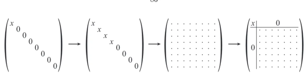
We assume that there are interaction terms in the Hamiltonian connecting the different factors of the Hilbert space. In §4.1 we provide a schematic representation of the evolution of the reduced density matrix, written in the pointer basis. When a bubble nucleates, some of the energy density that was in the potential for ϕ is converted to fluctuation modes.
Kniehl, “On the difference between the pole and MSbar masses of the top quark on the Electroweak Scale,” Phys. Salem, et al., “Boltzmann Brains and the Scale-Factor Cutoff Measure of the Multiverse,” Phys.

Higgs Potential and Decay Rates
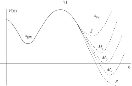
Let us begin by reviewing the stability of the Higgs potential, which depends on the behavior of the potential at large field valuesφ=|Φ|, where Φ is the electroweak (EW) Higgs doublet. How the universe develops depends on the value Λfar of the cosmological constant in the distant vacuum, where Λi= 8πGV(φi) andV(φEW)≈(2.3×10⁻³eV)4. The magnitude of bounceR will be the one that maximizes the decay rate, and µ≈R−1 is set to minimize the magnitude of the radiation corrections.
The larger contours show the 1σ and 2σ regions, using an alternative definition of the upper pole mass from CMS [ 63 ].
Cosmological Measures
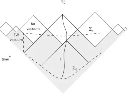
To achieve percolation, the life expectancy of an electroweak vacuum is equal to the actual age of our universe, Γdecay&H4[25]. The diamonds at the top of the diagram are the Minkowski terminal vacuum; if Λfar < 0, the lower boundaries of these diamonds represent singularities, and the diamonds themselves are absent. Dashed lines represent the causal part of the geodesic γ, depending on whether γ ends at the bubble wall or extends into Minkowski space.
If Λfar < 0, the interior of the bubble rapidly collapses to a singularity, terminating the geodesic γ.
Conclusions
Although a patch in the Hartle-Hawking vacuum is in a thermal state, it does not experience fluctuations in any meaningful sense. While it is true that an out-of-equilibrium particle detector inside the patch would detect thermal radiation, there are no such particle detectors floating around in the Hartle-Hawking vacuum. The cosmic no-hair theorem is given in the context of QFT in curved spacetime.
Even with horizon complementarity, there are no fluctuations in vacuum to lower entropy states as long as the larger Hilbert space is infinite dimensional.
Quantum Fluctuations vs. Boltzmann Fluctuations
- Decoherence and Everettian Worlds
- Quantum Fluctuations
- Boltzmann Fluctuations
If the device does not boot ready, we cannot be confident that it will ultimately be correctly correlated with the state of the system. Finally, we repeat the entire procedure, this time recording the measurement results in the second register of the device. This discussion assumes that the branching structure of the wave function can be discerned from the shape of the reduced density matrix for the macroscopic variablesHS.
In the last line the existence of the three branches is completely obscured; the reduced density matrix does not reveal which states of the system exist as part of different worlds.
Single de Sitter Vacua
- Eternal de Sitter
- Cosmic No-Hair
- Complementarity in Eternal de Sitter
Thus, we can try to define modes in de Sitter's asymptotic regions, I±, by analogy with Minkowski space. If the universe is in a Euclidean vacuum, the reduced density matrix describing the area within a causal horizon is thermal. We now turn to situations, like our universe today, in which the universe is not in a vacuum, but instead evolves in time.
6 As already mentioned, the massless case is problematic, since there is no de Sitter invariant vacuum in the non-interacting limit [107].

Multiple Vacua
- Semiclassical Quantum Gravity
- Complementarity in a Landscape
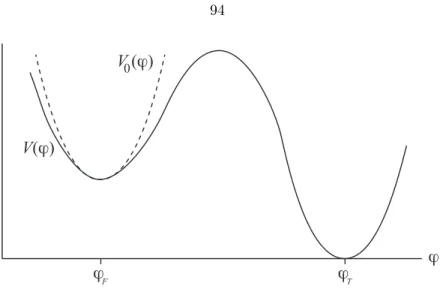
The dashed line represents the perturbative Hamiltonian for a false vacuum in which the potential is given by a local approximation to the true potential in the vicinity of ϕF. Nevertheless, we can consider the energy eigenstates of the perturbative Hamiltonian obtained by local approximation of the potential in the vicinity of ϕF as shown in the figure. HF−1 and HT−1 are the Hubble radii of the false and true vacuum, respectively, the latter being infinity in the Minkowski case.
In both cases, excitations can leave the apparent horizon in the false vacuum while remaining within the true horizon.
Consequences
- Boltzmann Brains
- Landscape Eternal Inflation
- Inflationary Perturbations
- Stochastic Eternal Inflation
- Other Formulations of Quantum Mechanics
They serve as an environment that we can trace to understand the state of the observable large-scale disturbances. Fluctuations only become real when they evolve into different decoherent branches of the wave function and generate entropy. But precisely in the slow-roll regime, where the stochastic inflation story is invoked, there is no entropy production, no measurement or decoherence, and no branching of the wave function.
The vacuum state of a scalar field is not a state of a definite field value, although it is centered around a potential minimum.

Conclusions
Quiros, “Improved Higgs mass stability bound in the standard model and implications for supersymmetry,” Phys. Wald, “Asymptotic behavior of homogeneous cosmological models in the presence of a positive cosmological constant,” Phys. Zurek, "Pointer Basis for Quantum Apparatus: In Which Mixture Does the Wave Packet Collapse?", Phys.
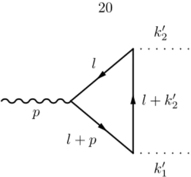
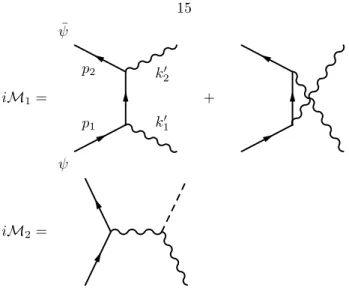
Tree-level dark matter annihilation
Ladder diagrams for dark matter annihilation and scattering
Dark Higgs decay
Dark gauge boson decay
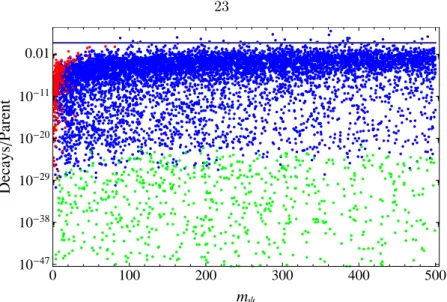
Parameter space scan
Number of A decays
Example: Parameter plots
Example: Annihilation and scattering cross sections
Example timeline for SU(N ) theory in AMSB without connectors
Example timeline for SU(N ) theory in AMSB with connectors
Glueball dark matter for SU(N ) theory
Region of interest for the scattering cross section
Mostly glueballino dark matter for SU(N ) theory in AMSB without connectors
Mostly glueball dark matter for SU(N ) theory in AMSB without connectors
Mixed dark matter for SU(N ) theory in AMSB without connectors
Glueballino dark matter for SU(N ) theory in AMSB with connectors
Schematic of the Higgs potential
Stability regions for the electroweak vacuum
Conformal spacetime diagram for our universe
Schematic evolution of a reduced density matrix in the pointer basis
Conformal diagrams for de Sitter space
Scalar field potential with multiple local minima
Conformal diagrams for de Sitter space with a false vacuum
Potential supporting different kinds of inflation