Damage evolution in uniaxial SiC fiber reinforced Ti matrix composites

(1)

DAMAGE EVOLUTION IN UNIAXIAL SiC FIBER REINFORCED Ti MATRIX COMPOSITES

Thesis by Jay Clarke Hanan

In Partial Fulfillment of the Requirements for the Degree of

Doctor of Philosophy

California Institute of Technology Pasadena, California

2002

(Defended June 18, 2002)

(2)

(3)

Acknowledgments

Several people have been helpful in bringing me to this point. The top of my list is clearly occupied by Robin. She is much more than my wife exemplifying the noble character many others never achieve. Of course, when considering family, I must be grateful to my parents Russ and Jan who continually encouraged creativity.

It was my undergraduate physics professor and academic advisor, Dr. Lynn Feuerhelm, who encouraged me to consider graduate school. I would not be here without him or the fateful meeting of John Rousseau who like so many other members of the Caltech community represented it favorably to a receptive undergrad looking for the right opportunity.

Dr. Ersan Üstündag has been extremely helpful as my academic and research advisor. He took a chance with me as I did with him, being his first student. Even though we have not agreed on everything, we would agree the chance was worth it. He always considered my opinion and was so instrumental in getting us to this point, which when I started down this path five years ago seemed far away. Looking back through this now seemingly short time, we have both grown first in science and never least in friendship. It was Dr. Üstündag’s contacts, including

Bjørn Clausen of LANSCE at Los Alamos National Lab who was extremely helpful with the FEM work; irreplaceable Dr. I. Cev Noyan of the IBM Watson Research Center who was such an inspiration contributing valuable advice and resources (including his load frame); Jon Almer and Ulrich Linert of the APS who helped facilitate the majority of

(4)

the relevant data collection and analysis; and Irene Beyerlein, also from Los Alamos, providing support with the micromechanical modeling,

which helped make up the army of people necessary to complete this work. There were also several graduate students who were helpful during the experiments where we not only tested materials, but ourselves (especially after sleep deprivation), namely: Geoff Swift, Stefen Kaldor, and Can Aydiner. I also have to thank Kevin Foltz who along with my sister Rae and daughter Raevan unknowingly challenged me to finish sooner rather than later.

I am also grateful to Dr. H. Deve at 3M Corp. for providing the specimens and helpful discussions about the properties of Ti-SiC composites. This study was supported by the National Science Foundation (CAREER grant no. DMR-9985264) at Caltech and a Laboratory-Directed Research and Development Project (no. 2000043) at Los Alamos. The work at the Advanced Photon Source was supported by the U.S.

Department of Energy, Office of Basic Energy Sciences (contract no. W-31-109-ENG- 38).

(5)

Abstract

Damage Evolution in Uniaxial SiC Fiber Reinforced Ti Matrix Composites

by Jay Clarke Hanan

Fiber fractures initiate damage zones ultimately determining the strength and lifetime of metal matrix composites (MMCs). The evolution of damage in a MMC comprising a row of unidirectional SiC fibers (32 vol.%) surrounded by a Ti matrix was examined using X-ray microdiffraction (µm beam size) and macrodiffraction (mm beam size). A comparison of high-energy X-ray diffraction (XRD) techniques including a powerful two-dimensional XRD method capable of obtaining powder averaged strains from a small number of grains is presented (HEµXRD²).

Using macrodiffraction, the bulk residual strain in the composite was determined against a true strain-free reference. In addition, the bulk in situ response of both the fiber reinforcement and the matrix to tensile stress was observed and compared to a three-dimensional finite element model. Using microdiffraction, multiple strain maps including both phases were collected in situ before, during, and after the application of tensile stress, providing an unprecedented detailed picture of the micromechanical behavior in the laminate metal matrix composite.

Finally, the elastic axial strains were compared to predictions from a modified shear lag model, which unlike other shear lag models, considers the elastic response of both constituents. The strains showed excellent correlation with the model. The results confirmed, for the first time, both the need and validity of this new model specifically

(6)

developed for large scale multifracture and damage evolution simulations of metal matrix composites. The results also provided unprecedented insight for the model, revealing the necessity of incorporating such factors as plasticity of the matrix, residual stress in the composite, and selection of the load sharing parameter.

The irradiation of a small number of grains provided strain measurements comparable to a continuum mechanical state in the material. Along the fiber axes, thermal residual stresses of 740 MPa (fibers) and +350 MPa (matrix) were found.

Local yielding was observed by 500 MPa in the bulk matrix of the composite. Plastic anisotropy was observed in the matrix. The intergranular strains in the Ti matrix varied as much as 50%. In spite of this variation, the HEµXRD² technique powerfully provided reliable information from the matrix as well as the fibers.

(7)

List of Illustrations and Tables

Figures

Number Page Figure 1-1 Some example views of continuous fiber metal matrix composites... 22

Figure 2-1 Photograph of adapted Fullam load frame on the goniometer at the 7.3.3 microdiffraction beam line at the Advanced Light Source. In this orientation, the open face of the load frame allows X rays to reflect from the surface of the sample. ... 33 Figure 2-2 Schematic of the diffracted beam position and the position of receiving

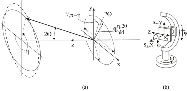
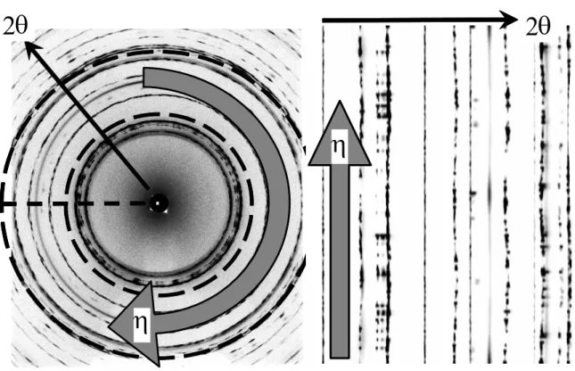
slits... 36 Figure 2-3 (a) Scattering geometry of a synchrotron experimental setup. x, y, z define the laboratory coordinate system, z being parallel to the incident beam, x is in the horizontal plane pointing outwards from the storage ring, and y is perpendicular to both z and x. The scattering vector q and the diffracted beam for a diffracting grain are indicated by solid arrows. Note that all scattering vectors coinciding on a cone with large opening angle (indicated by the dashed scattering vectors) are detected simultaneously on an area detector... 40 Figure 2-4 Diffraction patterns constructed from a θ/2θ scan with an analyzer crystal at 25 keV (left) and using a strip of pixels along η = 0 from an image plate exposure at 65 keV (right). Notice the peaks are much narrower with fewer data points, marked by an “o,” in a peak using the analyzer crystal, but the image plate scan takes less than 1/8^th the time and includes information from all η. (See Section 4- 2 for a fully indexed pattern.) ... 41 Figure 2-5 The image plate, initially exposed with rings in a radial format (left), is

converted to a Cartesian format (right) for analysis. ... 46 Figure 2-6 A zoomed-in view from two exposures of the image plate on the Ti-SiC

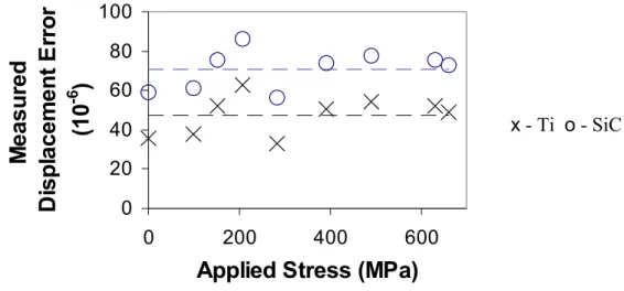
laminar composite (see Figure 2-5 for coordinates). The first (top) is at 0 MPa applied stress, the second at 850 MPa. Axial strains appear as shifts between the two frames directly at η = 0ô, 180ô and 360ô. Transverse strains are visible at η = 90ô and 270ô. For all other η the strain is a combination... 49 Figure 2-7 The translation error vs. applied load corrected for in the Ti-SiC composite.

An internal Si standard powder on the composite surface provided this information... 50 Figure 3-1 Finite element model (FEM) geometry and predictions of elastic strains at 650 MPa applied composite stress (along fiber axis, i.e., the z direction). (a) Mesh used in the FEM calculations. (b), (c) and (d) Normal strain distributions along the x, y and z directions, respectively. In (b) and (c), significant transverse strain gradients are observed across the specimen thickness. There is no variation in the

(10)

longitudinal elastic strain in the fiber (d), but there is some variation in the matrix due to predicted plastic deformation around the fiber. Average longitudinal strains in the fibers due to the applied stress alone are around 3040 µε while they are about 3110 µε in the matrix.. ... 53 Figure 3-2 A representative finite element mesh from the MSSL model for a laminar

fiber composite (adapted from [34])... 59 Figure 3-3 Schematic of crack geometries under consideration (adapted from ref. [34]).

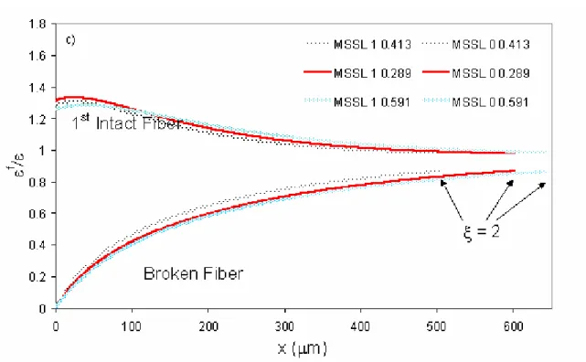
(a) Case (i): two fibers are broken but the crack-tip matrix regions are intact. (b) Case (ii): in addition to two broken fibers, the crack-tip matrix regions are also broken. Components are numbered with index “n”... 60 Figure 3-4 a) Case (i), and case (ii) with ρ = 0.289 for both one and two broken fibers.

b) Comparison of each predicted relative strain value for each ρ value assuming two fiber breaks and case (ii). Under case (ii) for the first intact fiber next to the break ε^f/ε is greatest for ρ = 0.591, while it is least for ρ = 0.289. c) Under case (i) for the first intact fiber next to the break ε^f/ε is greatest for ρ = 0.289, while it is least for ρ = 0.591. Case (ii) and (i) refer to strain profiles for fibers with and without failure in the matrix adjacent to the fiber break, respectively. ... 67 Figure 4-1 Scanning electron microscope (SEM) image of a typical specimen cross

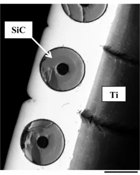
section. The fibers are 140 µm in diameter and are almost uniformly spaced with an average center-to-center distance of 240 µm. The carbon core of the SCS-6 fibers is visible as the dark circle in the center of the fibers. Two shades of SiC are also visible in the fiber corresponding to the two stages of SiC growth in manufacturing. The final dark ring around the fiber results from a protective carbon coat applied to the finished fiber. The cracks observed in some fibers occurred during specimen preparation. The total specimen thickness is about 200 µm. The shallow grooves seen in the Ti matrix are a result of the composite processing. ... 71 Figure 4-2 Schematic showing the composite geometry used in bulk XRD

experiments. The composite thickness was 0.2 mm. Fiber positions are represented by white lines within a gray matrix (for illustration only – not to scale). ... 72 Figure 4-3 Photograph of the experimental setup used for the 25 keV measurements.

The dashed line represents the transmitted and diffracted beam paths. The labels are as follows: (1) receiving slit, (2) Si diode beam stop, (3) translation stage, and (4) φ stage. θ and 2θ rotate about the y axis as shown by the curved arrow. See also Figure 2-3 b. ... 74 Figure 4-4 Indexed diffraction pattern for a θ/2θ scan of the Ti/SiC composite using a 2 x 2 mm² X-ray beam at 25 keV and a point detector. ... 75 Figure 4-5 Photograph of the high-energy experimental setup. The incoming and

transmitted beam path is represented by the dashed line. The image plate (1) is 1111 mm from the sample. A Si diode (2) acts as a beam stop also capturing the transmitted intensity. The translation stage (3) supports the load frame in a

(11)

horizontal position as opposed to the vertical position shown in Figure 4-3. An ion chamber connected to the incoming beam pipe (4) measures the intensity of the incoming beam, I0. ... 76 Figure 4-6 The strain gage (small circles with a connecting line) reveals drift of strain with time associated with the relaxation of load from a typical constant displacement load step. The strain in the matrix with its associated error given by the least squares refinement is shown by the flat line. Information from the entire 2θ scan (marked by arrows) is included in the refinement. The strains given by the Ti (11^.0) and Ti (10^.2) is given by the “x” and the “*,” respectively. These along with the strain from the SiC (220) peak, a “o,” are shown at the position the peaks occur in time. ... 79 Figure 4-7 Comparison of experimental strains from bulk with FEM predictions of

applied composite stress vs. average elastic axial strains in the first undamaged Ti- SiC composite during a loading/unloading cycle. Strain gage values are shown together with lattice strains in the Ti (10·2), Ti (11·0) and SiC (220) reflections obtained from diffraction. Thermal residual strains are included (see Table 4-1).

Note that due to load drifts not every stress level could yield suitable data for Rietveld refinement... 84 Figure 4-8 The macroscopic stress vs. strain in the first loading cycle of the second

undamaged composite along the fiber direction according to strain gage data (symbols). Deformation in the composite was elastic up to at least 700 MPa with very little plastic deformation even after 800 MPa. A line from a linear regression fit to the elastic portion of the curve is plotted over the data points to help illuminate the slight deviation from linearity in the strains caused by plastic deformation... 86 Figure 4-9 Elastic bulk strains in the fiber (a) and matrix (b) for increasing applied

tensile stress in the second cycle (symbols) on the second undamaged composite.

As before, the stress is applied along the fiber axial direction (axis 1). The FEM prediction for the loading cycle in the composite is also shown (lines). As in Figure 4-7 there is good agreement with the model up to the higher stresses. The deviation near 800 MPa signals the onset of global plastic strain in the matrix. An early onset of plasticity is observed in the transverse (ε22) direction where individual grains naturally show larger variations in strain (see text). (Strains are taken from the matrix (10^.2) diffraction ring and the fiber (220) diffraction ring.)

... 89 Figure 4-10 Strains during the release of applied tensile stress in the second

undamaged composite. The arrows show the direction of unloading. The fibers (a) show an overall linear behavior with very little average shear strain over the range of applied stress. However, the matrix (b) appears to deviate from linear behavior particularly in the transverse (ε22) and the shear (ε12) directions... 91 Figure 5-1 Optical micrograph illustrating the exposed fibers around the damage zone.

The red numbered line is parallel to the fibers with the red numbers displaying the approximate scale for some axial positions where strains were measured... 99

(12)

Figure 5-2 Schematic showing the damaged sample geometry used in the XRD experiments. The composite thickness was 0.2 mm. Fibers positions are represented by white lines within a gray matrix. The region etched is marked by an oval below the strain gage (for illustration only – not to scale)... 100 Figure 5-3 An SEM image at a 45^o tilt angle of the hole cut by EDM in the second composite. The hole cut completely through one fiber which was later assigned the label D. Beside it is fiber E which was partially cut. The matrix between these fibers is obviously cut as well as some of the matrix adjacent to D, the completely cut fiber... 102 Figure 5-4 Two photographs of the etched composite during the process of making the strain-free reference (before the fibers were etched away from the matrix). The thermal residual strains are strikingly apparent from this image. Once the fibers were freed from the matrix both phases returned to their originally flat configuration. A razor blade is also shown to provide scale. ... 104 Figure 5-5 Diagram of the low-energy microdiffraction technique. 2θ is in the same direction as θ... 106 Figure 5-6 Contour plot of Ti (20^.3) reflection from microdiffraction. The Cu (311)

reflection, which is close in d to the Ti reflection, exposes the Cu marker as the rough triangle between grains 13 and 14. The rectangle in the center of the figure borders the region scanned at higher ψ's. ... 108 Figure 5-7 Comparison of the macrobeam, , and microbeam, x, low-energy

measurements... 112 Figure 5-8 Absorption contrast image of the damaged region in the first composite as captured by the Si diode. Intensity is proportional to absorption, i.e., the darker a region the higher the absorption. The contrast is primarily due to Ti thickness.

The low density SiC fibers do not reveal features such as cracks. The absence of matrix from the surface of the sample near the damage region is evidenced by the bright region near the center of the image. The periodic change in intensity along y corresponds to the position of SiC fibers in the matrix. The fibers examined are labeled by number. Matrix regions examined lay between the labeled fibers.... 116 Figure 5-9 Map of β-SiC (220) reflection indicating the location of the buried fibers.

The oval outlines the damaged region. Fibers are numbered to indicate their location with respect to the damage zone (at the beginning, “Fiber 0” was broken).

It is interesting to note that the 30 x 30 µm² beam size used in this experiment yielded a continuous map for SiC confirming its small grain size. ... 117 Figure 5-10 Map of α-Ti (11^.2) reflection indicating the location of diffracting Ti

grains. The marked damage zone and fiber locations are visible from the dashed lines available from the transmission data collected simultaneously during the scan. With an average Ti grain measuring 29 µmacross, few grains are oriented for diffraction at a given θ angle. The damage zone marked by the arrow was etched to expose fibers... 118

(13)

Figure 5-11 The position of diffracting α-Ti grains that contribute to the intensity of the (10^.2) reflection using a 10 x 10 µm² X-ray beam. Since 9.1 keV X-rays are used, the examined grains are restricted to the surface of the sample. Both sides of the Ti matrix reference specimen were examined so that a layer of grains is exposed at the surface and the midplane of the sample (see Section 5-2 for description of the matrix reference). A photograph of the midplane surface is shown to the left of the contour plot. The layer at the midplane is also marked with what were fiber centers (between the black dashed lines marking the position the fibers were removed from) and matrix centers (between the grey dotted lines).

The white horizontal lines are an artifact common to synchrotron analysis. ... 120 Figure 5-12 A map of the positions sampled for fiber and matrix strains using the

image plate method on the second damaged Ti-SiC composite. Each of the 10 fibers was given a label “A” through “J”. Matrix positions are labeled “a” through

“i”. A hole was cut in fiber D and its neighborhood using EDM and is marked with an oval. The axial positions at +/-1.43 mm provide information for the far- field strains. Time constraints prevented collecting data from each position on this map. Relevant subsets were examined at each applied stress and are shown separately. ... 122 Figure 5-13 The intensity of the transmitted 90 x 90 µm² beam at 65.3 keV reveals the position of the fibers, grey columns, and the hole cut in the second damaged composite, a bright spot. Each of the 10 fibers is labeled on the x axis. The y axis provides the “Fiber Axial Position” which corresponds to the sampling position shown in Figure 5-12 numbered from the center of the hole outward in 75 µm steps. The first fiber, A, and neighboring matrix region were examined with a smaller 30 x 30 µm² beam giving rise to the lower transmitted intensity before fiber B. ... 123 Figure 5-14 Photograph of the load frame mounted on the goniometer in hutch C

downstream from 1-BM (bending magnet 1) at APS. The sample with a hole is shown in the grips. See inset (marked by blue rectangle) for a close-up of the composite. Placement of the strain gages is also visible in the image. The Si standard powder is mounted on the upstream side (back side in this image) of the sample. ... 124 Figure 5-15 The elastic residual strains in the fibers and intervening matrix regions as a function of axial position and fiber number for the damage zone of the first composite. The shade of each square depends on the value of strain measured using the 90 x 90 µm² beam at that position. Squares containing an “X” denote matrix positions where grains were not favorably oriented for diffraction. The position of the damage zone can be read from the relaxed (near 0) residual strains.

... 127 Figure 5-16 Example of diffracted peaks obtained from the matrix using the

microbeam and a point detector. The weak reflection shown here contributed to an “X” for the cluster of 3 in the upper right corner of Figure 5-15. Its signal to noise is too low for adequate fitting. The background intensity is the same for both peaks. ... 128

(14)

Figure 5-17 Residual fiber axial strain as a function of fiber axial position for the 5 fibers near the etched damage zone in the etched composite. Fiber 0 was broken before applying load. The change in strain for the fibers as a function of axial position is a result of matrix etched from above the fibers. The dashed line shows the strain given by the control fiber far from the damage region. ... 129 Figure 5-18 Residual matrix axial strain as a function of fiber axial position for the 4 matrix regions between the 5 fibers examined in the first composite. Both the action of etching away matrix from the surface and breaking the fiber acted to create the observed residual strains. The change in error bar length is associated with the presence or absence of diffracting grains. The strains given by the control matrix region are marked by the dashed lines. ... 131 Figure 5-19 For each fiber examined (D through J), the transmitted intensity measured by a silicon diode divided by the incident intensity measured by an ion chamber is plotted for each axial position sampled along the fiber. The fiber positions are identified by the lighter shade, more transmission, and the thicker matrix regions by the darker shade associated with less transmission. The hole appears the brightest. The axial position spacing is 0.075 mm except for the two extreme “far- field” positions, +/-12, which were an additional 0.6 mm from the previous point (Figure 5-12)... 133 Figure 5-20 The axial residual fiber strain as a function of fiber axial position for fibers D through H. The “far-field region” marked by an oval will later be used to normalize the fiber strains to compare with a micromechanical model. Two more fibers, I and J, (not shown) were similar to H. The error bars are smaller than the data points for all but two points near the hole on fiber D. The poorer statistics available from these positions is due to less diffracting material in the beam. ... 134 Figure 5-21 A contour plot of the matrix axial elastic residual strain for the regions

associated with the fibers, marked by the fiber label, and between the fibers. The presence of the hole around axial position 0 diminishes the residual strains in the matrix around fibers D and E. Even at regions distant from the hole, variation is present in the matrix residual strains. Compare spatial resolution with Figure 5-15. ... 135 Figure 5-22 The axial residual matrix strain as a function of fiber axial position for the regions between fibers D through J. The effect of cutting the matrix is primarily visible in the matrix between fibers D and E. The other matrix regions show fluctuations in strain, but since they are also observed far from the hole, they were due to possible spatial variations in processing and/or intergranular stress. The image plate clearly improves the ability to observe matrix strain (compare with Figure 5-17). ... 138 Figure 5-24 Matrix transverse residual strain from the α-Ti (10^.2) peak. Residual

compressive strain (dark shade) was observed between the fibers and residual tensile strain (light shade) was observed in the matrix above and below the fibers (marked by the “Fiber Label” positions). ... 139

(15)

Figure 5-24 a) The FEM prediction from Figure 3-1 with a solid and dashed arrow along the border of the plot exposing from where the solid and dashed lines for part “b)” were taken. b) Transverse thermal residual strain predicted in the composite by FEM. A center line along the fiber from the midplane of the composite to the surface shows tensile strain in the matrix (solid line). The transverse strains in the matrix centered between the fibers is compressive (dashed line). ... 141 Figure 5-25 Damage evolution under tensile load at the crack plane (x = 0 in Figure 5-1). Applied stress is plotted against applied axial lattice strain in the five fibers around the damage zone. At the beginning of loading, only fiber 0 was broken.

When the stress/strain profiles of the intact and initially broken fiber are compared, it is obvious that fiber +1 broke between 90 MPa and 430 MPa... 144 Figure 5-26 Applied strain in the first nearest neighbor fiber to the natural break (fiber +2, first damaged composite) for each load as a function of the axial position in the fiber. Load transfer (increase in strain compared to the far-field) from the broken fibers is realized even at the smaller load and continues to increase its magnitude and breath as the load increases... 145 Figure 5-27 Applied strain in fiber +1 which naturally broke while loading the first

damaged composite. The fiber shows a clear decrease in strain at the break plane.

... 146 Figure 5-28 Applied strain in the initially broken fiber as a function of axial position from the break. The wider profile observed in this fiber’s strains compared to the naturally broken fiber are due to the extent of initial damage in the fiber. (Data also from the first damaged composite.)... 147 Figure 5-29 Similar to fiber +2, the strains in the fiber which was a first nearest

neighbor to the initially broken fiber as a function of axial position from the break are shown. The load transfer is first apparent at the smaller applied stress and increases with increasing stress. The profile looses symmetry with the break plane due to the damage profile in its neighbor (Figure 5-28). (Data also from the first damaged composite.) ... 148 Figure 5-30 Applied strain in the second nearest neighbor fiber to the break (fiber -2) for each applied load as a function of the axial position in the fiber. An effect from the broken fibers is realized even at the smaller load and continues to increase its magnitude and breath as the load increases. (Data also from the first damaged composite.) ... 149 Figure 5-31 Contour plot of the strains at the maximum applied stress (530 MPa) for all the fibers examined in the first damaged composite. The relative position of stress transfer from the break to the intact fibers is clear. The data here is taken from the last applied stress shown in Figure 5-26, Figure 5-27, Figure 5-28, Figure 5-29, and Figure 5-30... 150 Figure 5-32 Each box represents a position analyzed with the 90 x 90 µm² beam. The fibers A-J and neighboring matrix regions were analyzed in the configuration shown. These positions are a subset of the positions analyzed before stressing the

(16)

composite (Figure 5-12). The numeric label for the positions used in the strain contour maps is shown on the right of the figure. For reference, the position of the hole cut in the composite is also shown in the figure. ... 151 Figure 5-33 A strain map of the total elastic axial strains (residual + applied) in the

fibers for the composite with a hole at 850 MPa applied stress. The hole is marked as a square since no matrix regions are shown. The strains reveal a decrease in strain near the hole for the broken fibers D and E with the first nearest neighbor fibers C and F compensating with larger strains. The rest of the fibers show strains around 0.11%. Compare with Figure 5-31 prepared from the point detector data... 152 Figure 5-34 The applied axial strains (total strain (Figure 5-33) minus the residual

strain (Figure 5-20)) for the fibers D through I are shown for the 850 MPa applied stress. The width of the hole is marked on the graph for fiber D. The spatial resolution and strain resolution have both improved compared to the etched composite previously examined with the point detector. The data point on fiber D taken inside the hole showed less intensity, and therefore a greater error than the other positions... 153 Figure 5-35 A contour map of the total elastic axial strains in the Ti matrix for the

composite with a hole at 850 MPa. The fiber positions are labeled and separated from the “matrix only” columns by dashed grid lines. The broken fibers appreciably affect axial matrix strains two fiber diameters from the break. Such a figure with continuous strain information from the matrix cannot be constructed from the point detector results. ... 154 Figure 5-36 A map of the total elastic shear strains in the Ti matrix of the composite with a hole at 850 MPa. The effect of load on the hole is observed in the stress concentrations around the hole. Arrows follow the path of maximum shear away from the hole... 155 Figure 5-37 A strain map of the total elastic transverse strains in the matrix of the

composite with a hole at 850 MPa. The strain at each fiber location is tensile but the strain between each fiber is on average compressive. ... 156 Figure 5-38 A typical shift (90 µm) in the axial position of the hole referenced to the laboratory coordinate system due to changing the load on the composite. The transmitted intensity along fiber D normalized by an incoming beam monitor allows alignment in the fiber axial direction. Alignment in the transverse direction may be performed through monitoring the intensity change along the fiber radius (not shown). ... 159 Figure 5-39 Total matrix axial residual strain around the hole after loading and

unloading the composite from 850 MPa. The position of the hole in the composite is marked with an oval. The region marked by the “X” was not sampled due to time constraints... 160 Figure 5-40 Matrix transverse residual strain around the hole after loading and

unloading the composite from 850 MPa. The position of the hole in the composite

(17)

is marked with an oval. The position labeled “X” was not sampled due to time constraints. ... 161 Figure 5-41 Matrix residual shear strain after loading and unloading the composite

from 850 MPa. The position of the hole in the composite is marked with an oval.

The arrows connect the points of maximum shear strain traveling away from the hole. As with the plots above, the position labeled “X” was not sampled due to time constraints... 162 Figure 5-42 Strain map of the change in matrix axial residual strain due to loading (to 850 MPa) and unloading the second composite. The matrix over the broken fiber, D, is the first column on the left of the map. The darker regions identify locations of greater plastic deformation while loading the composite... 164 Figure 5-43 The change in axial residual strain for the first two matrix columns

illustrates the contrast between the two regions. Near the plane of the broken fiber significant deformation from the 850 MPa applied stress occurred in the intact matrix column e. Since matrix column d was broken it could not carry load and consequently did not significantly deform near the break... 165 Figure 5-44 The significant change in fiber residual axial strain for fiber E, which

broke under the application of load. Permanent deformation in the matrix above and below the fiber which deformed as a result of the strain associated with the break is also revealed by the analysis. ... 166 Figure 5-45 Change in axial strain for fibers D and F. The axial strain does not change near the free surface for the cut fiber D. In contrast, the intact fiber F shows a significant change in residual strain upon unloading due to permanent deformation in the matrix... 167 Figure 5-46 Change in axial strain for the two fibers furthest from the break. Change in the axial matrix strains at these fiber locations is shown as well. ... 168 Figure 5-47 Change in axial elastic residual strain for fiber G. Though similar to the above fibers far from the break, the position sampled to the immediate negative side of the crack plane showed no change in strain—the sign of a poorly bonded interface. Adding support to the observation, a local increase in plastic deformation was observed at the same location through the change in matrix strain... 169 Figure 5-48 Comparison of strains from the MSSL model predictions (case (i) the

black line and case (ii) the grey line) and XRD data from fibers (symbols) in the first damaged composite: (a) The two broken fibers; (b) the second intact fiber;

(c) first intact fibers. The applied tensile stress decayed from 430 to 410 MPa for one applied stress and 530 to 540 MPa for the other applied stress shown. The model calculations were performed for ρ = 0.591. Strains were normalized with respect to the averaged applied far-field value (the average strain for all |ξ | > 4).

Particularly for (c) the first intact fiber, case (i) with two broken fibers (0 and +1) gives the best agreement with model predictions. The expansion of the profile for fiber 0 is due to the width of initial damage in the fiber... 175

(18)

Figure 5-49 Comparison of normalized strains from MSSL model predictions and XRD data from the matrix in the first damaged composite for case (i)—intact matrix at crack tips. (a) Depicts the matrix region between the two broken fibers (0 and 1), (b) the matrix region between an intact and broken fiber (−1 and 0), (c) the matrix region between two intact fibers (−2 and –1), and (d) also a region between an intact and broken fiber (2 and 1). The applied tensile stress under constant displacement drifted from 450 to 430 MPa. The model calculations were performed for ρ = 0.591. Strains were normalized with respect to the applied far- field value, ε^m = 2340 to 2240 µε. Elastic strains for each region of the matrix examined are plotted against the best-fit model predictions for that region. Grain- to-grain strain variations are significant here as few grains represent each position.

... 176 Figure 5-50 Illustration of the interpretations of composite geometry relevant to the

MSSL model. Since the model only considers matrix between the fibers and the real composite has matrix all around the fibers, the definition of the width of matrix between the fibers W has multiple interpretations. One simplification of the geometry assumes the fiber cross section is square (dashed line). This simplification conveniently results in constant width between the fibers throughout the thickness... 178 Figure 5-51 Normalized relative strains in the fibers around the hole from the 850 MPa maximum applied stress to the composite (symbols) compared to the MSSL model predictions for the second geometrical version of the model above (lines). More stress is transferred to fibers F and G than predicted by the MSSL model which is due to plastic deformation in the matrix (see next figure)... 181 Figure 5-52 Normalized relative axial strains in the matrix from 850 MPa maximum applied stress to the composite around the hole. The MSSL model predictions for the second interpretation (ρ = 0.290) are shown (lines) compared to the measured strains (symbols). At this applied stress the matrix has begun to yield, particularly near stress concentrations as would be found by the hole in “e”. The normalized matrix strain never exceeds 1.3. Yielding begins at the interface and transfers load to the fibers (Figure 5-49)... 182 Figure 5-53 A comparison of the MSSL model predictions (lines) for the unloading

fiber strains in the second damaged Ti-SiC composite (with a hole) for fibers B-D (symbols). The hole in fiber D was approximated by a series of breaks. The overall fit improves by averaging the distance between the fibers for W and reducing the thickness in the model to the average thickness of the fiber (solid line). The dashed lines depict the model predictions if the minimum distance between the fibers is used for W and the matrix thickness is used for t. ... 184 Figure 5-54 A comparison of the MSSL model predictions (lines) for the unloading

fiber strains in the second damaged Ti-SiC composite, with a hole, for fibers E-F (symbols). Fiber E broke naturally but its strains show evidence of the neighboring hole. Two extremes of the geometry provide the two model prediction shown (ρ = 0.290 (solid line), ρ = 0.667 (dashed line))... 186

(19)

Figure 5-55 A comparison of the MSSL model predictions (lines) for the unloading matrix strains (symbols) in the Ti-SiC composite with a hole. The dashed lines depict the model predictions if the minimum distance between the fibers is used for W and the matrix thickness is used for t (ρ = 0.667). Overall the fit improves by averaging the distance between the fibers for W and reducing the thickness in the model to the average thickness of the fiber (solid line, ρ = 0.290). Matrix c is damaged near the hole contributing to the strain falling short of the model prediction. ... 187 Figure 5-56 A comparison of the MSSL model predictions (lines) for the normalized unloading matrix axial strains (symbols) in the Ti-SiC composite with a hole. As above, the dashed lines depict the model predictions if the minimum distance between the fibers is used for W and the matrix thickness is used for t. Again, the overall the fit improves by averaging the distance between the fibers for W and reducing the thickness in the model to the average thickness of the fiber (solid line). Though possibly influenced by the debond in fiber G (Figure 5-54), matrix e strains fall short of the model prediction. ... 188 Figure 5-57 For completeness a final comparison of the MSSL model predictions

(lines) for the unloading matrix strains (symbols) in the Ti-SiC composite with a hole. As above, the dashed line depicts the model predictions if the minimum distance between the fibers is used for W and the matrix thickness is used for t and the solid line depicts the fit for averaging the distance between the fibers W and reducing the thickness in the model to the average thickness of the fiber. The general trend depicted by the model is observed... 189 Tables

Table 3-1 MSSL model predictions of the axial strain concentration factors (SCFs) in the first intact fiber at the crack plane (x = 0) for the Ti-SiC composite... 64 Table 4-1 Bulk residual axial strains in the Ti-SiC composite (from Figure 4-7)... 80 Table 4-2 Residual axial strain (10^-6) evolution in damage free Ti-SiC composites

averaged over all fiber and matrix regions in the beam. The first three rows correspond to measurements from the first composite examined with the point detector. The last two rows correspond to values taken from the second composite using the image plate. The second composite was also taken to a greater applied tensile stress. ... 94 Table 5-1 Averaged results of the microdiffraction analysis... 110 Table 5-3 The average axial strain in matrix regions between the fibers (lower case) and matrix regions located at the fiber (above and below, upper case). Total averages for each region are in bold. ... 136

(20)

(21)

1. Introduction

1-1. Background and Motivation

Metal matrix composites (MMCs) were introduced as structural materials in the early 1970s. Nearly a decade later, with improvements in processing, applications in aeronautics and the automotive industry began demanding materials with the specific strength and modulus, controlled toughness and thermal expansion coefficient, hardness, and an improved fatigue response only available from MMCs. Better understanding of their mechanical behavior fueled improvement of the reinforcements which in turn improved the composite properties. Consequently, MMCs have found a number of applications which now vary from sporting goods to thermal and wear-resistant parts [1, 2].

Of the various types of MMCs (short fiber, particle, or continuous fiber reinforced), the continuous fiber reinforced variety provides the highest structural performance.

These MMCs, usually reinforced with high modulus ceramic fibers, rely on the continuous fibers for their strength using the matrix primarily for protection and support of the fibers (see, for example, Figure 1-1). The matrix is also the key player for local stress transfer between fibers. The other types of MMCs typically depend on the weaker matrix to act also as a primary load bearing agent.

(22)

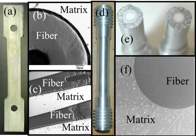
Figure 1-1 Some example views of continuous fiber metal matrix composites.

(a) Photograph of a two-dimensional continuous fiber metal matrix laminate composite tensile test specimen (Ti matrix/SiC fibers).

(b) Scanning electron micrograph (SEM) of the polished end of the same composite.

(c) Side view of a polished face of the laminar composite similar to that found in (a) here also using SEM.

(d) Photograph of a single fiber metal matrix composite (Al matrix/Al2O3 fiber).

(e) Fracture surface of a similar composite to (d) exposing the fiber.

(f) An SEM of the polished end of (d).

The transfer of load from a broken fiber to the rest of a composite as it is deformed is one of the fundamental micromechanical processes determining composite strength, lifetime and fracture toughness. It is a complex process that depends on fiber/matrix interface properties, the constitutive behavior of matrix and fibers, the geometric arrangement of fibers, fiber volume fraction, and fiber strength distribution. The

Fiber Matrix

Matrix Fiber

Fiber

Matrix Fiber

Matrix

(a) (b)

(c)

(d)

(e)

(f)

(23)

prediction of this process is further complicated since the in situ mechanical properties of the constituents are significantly different than the properties in the monolithic form [3, 4, 5]. These differences stem from (i) constraints imposed by neighboring phases; (ii) changes in microstructure due to altered processing conditions required for composite manufacturing; (iii) thermal residual stresses due to coefficient of thermal expansion (CTE) mismatch between different phases; and in some cases, (iv) high dislocation densities near the fiber/matrix interface [6].

Conventional stress analysis of fiber composites employs the use of strain gage rosettes on the surface of the matrix. Test methods such as the ASTM specification D3039-76 (1989) provide a detailed example of the traditional analysis which provides information on the longitudinal and transverse tensile strength, Young’s moduli, tensile strain, and major (longitudinal) and minor (transverse) Poisson’s ratios [7]. However, the macroscopic stress-strain curves obtained by these conventional means result from the co-deformation of the individual phases making it impossible to determine the phase- specific in situ constitutive behavior. Typical composite deformation includes collective nucleation and evolution of damage, fiber fractures, matrix fractures and plasticity, as well as interface separation and sliding.

Several mechanical models have been proposed to describe the behavior of MMCs.

The simpler models such as the concentric cylinder or the Eshelby model point to the fiber fraction as the more sensitive parameter determining a composites properties. Bulk properties have also been predicted with relative success using finite element modeling (FEM). Several efforts to improve computational speed over FEM have been proposed.

One of these, which uses the “shear lag” concept, will be examined in more detail in

(24)

Section 3-2. Reliable micromechanical models, particularly models that correctly predict ductility in MMCs, require further development [8].

Whatever model is employed to understand an MMC, there still remains an overwhelming need to validate or refute the predictions with relevant mechanical data.

Such data are in short supply. Modeling studies are often compared to predictions from Monte Carlo simulations [9, 10] or incomplete subsets of data [8 (p. 241)], limiting the ultimate relevance to the engineer who must deal with the real composite. In the Ti-SiC composite system, micromechanical studies applying acoustic methods have been used to identify in situ fiber breaks. But these studies do not provide the phase-specific strains in the matrix and fibers, and only hint to the mechanism of load transfer in the composite [11].

In order to predict the strength and lifetime of a fiber composite, the load transfer from broken fibers to the surrounding intact material must be understood. This requires accurate determination of stress-strain evolution at the scale of microstructure—usually on the order of the fiber diameter. In situ measurements of stress/strain can then be used to validate and refine predictive micromechanics models. In special cases, this has been achieved using optical methods such as micro-Raman and piezospectroscopy [for example: 6, 12, 13, 14, 15]. These studies provided valuable insight about fiber strains in damaged composites at length scales approaching several µm. However, in most of these studies either the matrix could not be characterized, or only shallow surface regions were investigated.

More general probes that measure both the matrix strain and the reinforcement strain are necessary to truly understand composite deformation. One such tool historically

(25)

useful in measuring stress is X-ray diffraction. Low-energy X-ray diffraction, on the order of 8 keV,^* has long been used to measure stress in single phase materials and, through several technological improvements, has become a standard method for measurements of residual stress in many materials [16, 17]. However, for most materials, low-energy X-ray diffraction provides information specific to the material surface. This is particularly true for MMCs where, beyond aluminum, the penetration depth of low- energy X-rays is on the order of micrometers (e.g., 30 µm for Ti at 9 keV) and rarely provides information on more than one layer of matrix grains. Destructive methods such as layer removal employed low energy X-rays for depth-resolved residual strain measurements [18, 19], but with the exception of diffraction via neutrons, observation of continuous fiber strains under applied stress was relegated to the abovementioned specialized cases where the matrix was optically transparent.

Neutron diffraction also remains a valuable tool in the investigation of MMC mechanical behavior. In-depth studies of the bulk composite response to applied stress coupled with phase-specific fiber and matrix strains have provided significant insight to the peculiar behavior of these materials [20, 21, 22, 23, 24, 25, 26, 27, 28]. Though one of these studies [28] does provide single fiber specific strains coupled with the elastic portion of the matrix response, the inherent advantage of the neutron’s penetrating depth through week nuclear interactions also limits the probe’s spatial resolution. In [28] the researchers compensate for this drawback by increasing the fiber diameter substantially beyond the realm of a typical MMC. The result is a measurement which is applicable to continuum mechanics models, but entirely avoids the role of fiber matrix interactions on

*Such as X rays available from a typical Cu tube.

(26)

the order of the microscale [29, 30]. Other more recent investigations have shown that, for a more traditional MMC even of the same material system, the fiber matrix interface is characterized primarily by abrupt variations in stress never considered by continuum mechanical models [31, 32]. Thus a general lack of information concerning MMC deformation mechanisms at the scale of the microstructure persists.

1-2. Approach

It naturally follows that a study on a practical high-performance MMC would be of significant value to the modeling and eventually engineering community. One such composite is the Ti-matrix/SiC-fiber laminate composite (Figure 1-1 (a)-(c)). Both Ti and SiC are well known as high-temperature structural materials [33]. Naturally, the Ti- SiC composite itself has received considerable attention from other researchers simply due to the performance characteristics of its constituents [8, 11, 19, 21, 23, 24, 25, 26].

However the fundamental lack of phase-specific micromechanical data remains.

The following describes the use of X-ray diffraction to determine the phase-specific in situ load transfer and damage evolution under applied tensile stress in a Ti-SiC composite. Synchrotron X rays were required to obtain the necessary intensity to reduce the beam size below the fiber diameter while maintaining sufficient diffraction statistics and strain resolution over reasonable count times. The technique described may be tailored to glean the specific mechanical information needed and is applicable to a variety of composites beyond the Ti-SiC system. Multiple scales from the micro (several µm) to macro (several mm) are simultaneously available with this method. No other technique, including neutron diffraction, could provide the spatially resolved strain resolution from

(27)

multiple phases so crucial to understanding mechanical behavior of metal matrix composites.

In this thesis, the Ti matrix and SiC fiber strains were compared to predictions from a general micromechanics model [34]. This “matrix stiffness shear lag” (MSSL) model accounts for the linear elastic co-deformation of fiber and matrix in a wide variety of unidirectional fiber composites containing any configuration of multiple fractures. This is the first damage evolution study tailored for application to a micromechanics model conducted on a continuous fiber MMC where both matrix and fibers were investigated simultaneously at the scale of the microstructure.

(28)

2. Diffraction Techniques to Study Composites

The following briefly introduces the use of X-ray diffraction to measure strain. Some issues concerning the application of stress to a diffracting body are also presented. The final section outlines the two primary analysis methods used to measure the strains in the Ti-SiC composite. The specifics of each experimental procedure are presented within the respective chapters regarding the experiments.

2-1. Strain and X-Ray Diffraction

Strain measurement with “traditional” X-ray diffraction (XRD) is a well-established technique [16, 17]. Measurements of strain using X rays were performed as early as 1925 [35]. Recent advances include the use of high-energy X rays (with more penetrating power) and microdiffraction with sampling volumes of several µm³. Both of these are best performed at synchrotron facilities, and a combination of which was used for this study.

Microdiffraction experiments such as [36] by Noyan and co-workers at the National Synchrotron Light Source (NSLS) achieved a spatial resolution of a few µm. Their systematic investigations of the instrument improved its accuracy and identified potential sources of error such as beam divergence and the sphere of confusion [37, 38]. They provided a portion of the substantial groundwork establishing microdiffraction as a viable XRD method.

The use of high-energy X rays to sample regions deep in materials has been demonstrated by a number of pioneering studies [examples: 39, 40, 41, 42, 43]. High- energy synchrotron XRD provides the ability to probe buried regions in materials. The

(29)

high intensity of synchrotron X rays also provides excellent time and spatial resolution.

The abovementioned synchrotron XRD studies employed both monochromatic [39, 41, 42], and polychromatic [40] beams with the former yielding higher strain sensitivity (10^-5 vs. 10^-3). They also sampled volumes as small as several hundred µm³. Although a few studies are noted on strain distributions around fibers in composites [39, 40, 41], none are known that investigated the in situ mechanical behavior of phases on multiple scales.

In general, direct XRD strain measurements under kinematic diffraction conditions are limited to crystalline phases of materials which deform elastically.^* Polycrystalline bodies deform when subjected to external or internal stress. As long as the stress is small, the deformation is reversible. This reversible deformation is elastic strain. The X- ray strain method requires a measurement of the lattice parameters, using a least-squares refinement of several peaks, or lattice spacings, specific to a single peak position, in the material.

According to Bragg’s Law, λ = 2 d sin θ, diffraction peaks arise at a particular Bragg angle, θ, determined by the lattice spacing, d, of the atoms of a lattice in a grain (or crystallite) which is oriented for the diffraction condition at a particular wavelength, λ.

Peak shifts determined as a difference in initial and final angles ∆(2θ) are proportional to changes in the average distance between lattice planes, ∆d [16]. It is this change in lattice spacing which provides the diffraction elastic lattice strain in a diffracting material:

ε d −d0

= d0 (2-1)

* It is possible to deduce plastic strain information using diffraction in a crystalline body or elastic strain information from an amorphous body (as a second phase), but here these are considered indirect strain measurements.

(30)

where d0 is the reference lattice spacing. When d0 is from a stress-free material, the resulting strain measured includes residual strain. Measuring residual strain using diffraction is well developed [17]. The choice of a strain-free reference and measurements of d0 will be presented in Section 5-2.

Although the procedure is simple to describe and understand, its appropriate application requires extreme care, especially when considering the level of accuracy required to measure strains.^* Errors can be intrinsic to the technique (and the instrument used) or they can result from the inhomogeneous nature of materials studied. In the general case when stress is applied to a polycrystalline material or composite, the total strain measured with diffraction at any point includes three terms [44]:

εijtotal = εijo + εijinter. + εijres. (2-2) where, εijo is the homogeneous elastic strain due to applied stress σ^o (if the material were a homogeneous isotropic body), εijinter. is the interaction (or coupling) strain due to elastic incompatibility or inhomogeneous plastic yielding, and εijres. is residual strain. Each of these terms is an average value over the sampling volume. Since not all the grains within that volume contribute to the diffraction pattern, effects from heterogeneity can become critical when sampling small volumes.

The measurement of a peak position to assign lattice spacing possesses an inherent error associated with fitting the peak. Depending on the source of the radiation and the conditions of the optics and specimen sampled, the peak width and profile will change.

While sensitive to lattice spacing, the peak position is also sensitive to the optical and sample geometric configuration. Each component possesses its own contribution to the

*Many materials yield or fracture before the elastic strain reaches 1% (typically 0.2% to 0.5%).

(31)

error in the final peak position. A good review of errors in strain measurements is presented in [17]. In summary, the best practice to minimize error in a diffraction experiment is to maximize the exposure time, minimize inadvertent sample translation from the center of diffraction, and use an internal standard. An internal standard may be composed of any suitable diffracting material not expected to change its lattice spacing over the course of the experiment. If systematic errors from sample displacement or other minor misalignments occur, a strain-free standard will show a peak shift which may then be used to correct for erroneous shifts in the strained sample [45]. Internal standards also allow samples scanned between alignments to be compared, a necessary option for reliable residual strain measurements.

Selection of an internal standard can be difficult. Consideration must be made for overlap in the peaks from the standard with the peaks from the specimen. There may also be problems with exposure times, as the peak intensity from a strain-free standard is usually much greater than a strained material due to texture, grain size effects, or strain broadening. The best standards are available from the National Institute of Standards and Technology (NIST); however, a well-characterized powder which provides peaks that do not appreciably overlap will generally suffice. Several common standard powders include: Al2O3, CeO2, LaB6, NaCl, and Si.

(32)

2-1.1. Strain Measurements with In Situ Mechanical Loading

With X-ray diffraction’s ability to measure strain, it follows to apply the analysis to a body under applied stress. Mechanical loading is not new to XRD. However, in spite of the considerable number of mechanical loading experiments performed using diffraction to measure strain, advances in optics and peripheral equipment have maintained a realm of continuous flux and renewal on the cutting edge of modern science. One significant new instrument planned for the Advanced Photon Source (APS) at Argonne National Lab, HEX-CAT (High Energy X-ray Collaborative Access Team) will dedicate much of its time to strain measurements using high energy X-ray diffraction. New instruments are also planned at other advanced facilities relying on neutron and X-ray diffraction (JEEP at Diamond/ISIS, ENGIN X at ISIS, VULCAN at SNS, SMARTS at LANSCE, a parallel optics µbeam line upgrade at X-20 (NSLS), and a 3-D spatially resolved sub-µm polychromatic beam line replacing 7.3.3 at ALS, to name a few).

The first mechanical loading experiments on unidirectional MMC composites performed by Caltech researchers using diffraction took advantage of the custom load frame based on an Instron hydraulic press at the Los Alamos Neutron Science Center.

Further experiments using a small custom load frame designed by I. C. Noyan (IBM) were performed using synchrotron XRD at APS. Modifications to the Noyan load frame and adaptation of an Scanning Electron Microscope (SEM) load frame designed by Fullam,^* have continued to improve the capability to mechanically load composites at Caltech while performing XRD measurements (see Figure 2-1, see also Figure 4-3, Figure 4-5, and Figure 5-14).

*Ernest Fullam Inc., 900 Albany Shaker Rd., Latham, NY 12110-1491.

(33)

Area Detector

Load Ce ll Load Ce

ll Incom

X-rays ing Area Detector

Load Ce ll Load Ce

ll Incom

X-rays ing

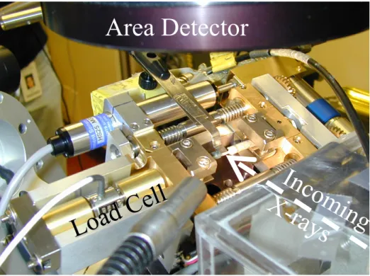
Figure 2-1 Photograph of adapted Fullam load frame on the goniometer at the 7.3.3 microdiffraction beam line at the Advanced Light Source. In this orientation, the open face of the load frame allows X rays to reflect from the surface of the sample.

As with any mechanical loading experiment, many factors including accurate load cells, a stiff frame, and stable strain increments are important in providing a good experimental tool. However, a load frame intended for use with diffraction also requires an open or transparent beam path exposing the sample to as wide a range of visibility as possible. Shadowing the beam by the load frame or grips limits the length of potential specimens, and since the diffracted beam averages strain over the irradiated area of the sample, edge effects and non-uniformities in the grip region should also be avoided. The weight of a load frame is often critical since, in general, it should be free to rotate when mounted on a traditional goniometer. For some special cases, very large goniometers or other robotic platforms are available to translate a massive load frame in the beam [28].

Finally, a constant stress mode as opposed to a constant strain or displacement

(34)

operational mode is preferred since diffraction measurements are associated with an exposure time sometimes approaching many hours.

When a constant load cannot be maintained, it is necessary to track the load over time and assign the appropriate load to each scan. Here “scan” refers to the measurement of one or more peak positions from a diffraction experiment as described below. In order to track the load on a sample mounted in an X-ray goniometer, a program was designed in LabVIEW^* 6i (see Appendix A). The load cell used was an Entran^† ELHS-T1M-1KL which requires a 10 to 15 V excitation to measure forces up to 6500 N. The output voltage from the load cell is proportional to the applied load on the sample.

Using digitization hardware, the output voltage can be read by a computer using the LabVIEW program. The time corresponding to the load cell reading by the computer is correlated with the start and end time of the scan. For a typical constant displacement experiment on metal matrix composites, the load does not change more than 0.1 MPa during short scans. However over the course of several scans the change can become significant enough to effect the strain measurements. Without appropriate accounting for this change in applied stress, strain results would be misinterpreted. A secondary link, assuring the scan times and load cell logged times are synchronized is also recommended.

When a scan starts, a digital pulse may be sent to the LabVIEW computer and logged on the data file with the applied stress values. The pulse is particularly useful for tracking the load during manual scans which may not be recorded at regular time intervals.

*The LabVIEW software is commercially available from National Instruments, 11500 N Mopac Expwy, Austin, TX 78759-3504.

†Entran Devices, Inc. 10 Washington Ave., Fairfield, NJ 07004-3877.

(35)

In summary, even over the last three years, significant improvements to mechanical loading methods coupled with diffraction strain measurements have occurred [29, 30, 31, 32]. The driving force for such improvements is difficult to define. One important factor is the investment in advanced diffraction facilities. SMARTS is a good example of recent improvements which were particularly clear as it stood next to a previous generation workhorse for neutron diffraction strain measurements, NPD [28].^* Similar advances such as the high-energy beam line at APS, have reduced the constraints on the application of mechanical load frames. Such synergistic combinations allow for high resolution X-ray strain measurements. A methodology for these experiments is presented in the following section.

*The Neutron Powder Diffractometer (NPD) was, as its name implies, originally dedicated to structure determination through powder diffraction. However it also, like many of its sisters, became a tool of the materials scientist.

(36)

2-2. High-Resolution X-Ray Strain Measurements.

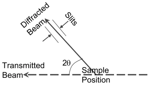
High-resolution X-ray strain measurements require precise knowledge of the relative diffracted beam position (Figure 2-2). The relative as apposed to the absolute diffracted beam position is of interest since strain is calculated from a difference in lattice spacings, Eq. (2-1), which would be accurate even if the absolute lattice spacings are precise but inaccurate. For X-ray strain measurements, the overall objective is to obtain a high 2θ spatial resolution over the range of interest. Receiving slits are a very common tool used to improve the 2θ resolution of a diffraction measurement (Figure 2-2). Very narrow slits potentially increase resolution but significantly reduce the signal intensity.

Slits Diffracted

Beam

2θ Sample Position Transmitted

Beam

Figure 2-2 Schematic of the diffracted beam position and the position of receiving slits.

For most X-ray diffraction systems, assuming total mechanical freedom to reduce the slit size, consideration for the available time to measure the intensity at a particular 2θ typically fixes the lower limit of the slit width. For example, using a common Cu tube X- ray source on a standard Siemens diffractometer, reducing the receiving slits to 0.3^o from

(37)

3.0 will extend an hour long scan into an overnight scan with similar peak intensity.

However, with the large number of photons (or flux) available from a synchrotron X-ray source, difficulties in manufacturing reliable narrow slits can also provide a lower physical limit. Methods to reduce the receiving slit aperture have many forms. Slits range from stacked plates, called Soller slits, to reduce divergence to pinhole slits with very small apertures or with large aspect ratios maximizing the 2θ resolution at the expense of divergence in the direction perpendicular to θ for a gain in throughput. These slits may also be stacked to reduce divergence. A maximum angle of divergence can be readily realized with simple geometry: for two slits a distance, S, apart, and aperture A;

the angle of maximum divergence, β, from a point source is 2 A / S. Since divergence broadens the peak in 2θ, the strain resolution will diminish with divergent beam optics.

However, particularly with synchrotron X radiation, the source may produce a highly parallel beam. For highly parallel optics, it is difficult and often unnecessary to mechanically construct slits which provide a significant reduction in divergence. In addition, parallel beam optics reduces the sensitivity to systematic errors. For parallel optics, the most effective “slit-like” tool to improve the 2θ spatial resolution is an analyzer crystal. Analyzer crystals consist of a single crystal which has rectangular trough or channel cut parallel to a diffracting plane through the length of the crystal. If properly aligned, the diffracted beam must diffract at least twice—once from each surface of the channel—to pass through the channel in the analyzer crystal before reaching the detector. Since it is a single crystal, the diffracted intensity is high, but only a narrow band—a subset of an incoming divergent beam—approximately the Darwin- Prins width [46], will diffract through the crystal for a given orientation. A peak position

(38)

measurement requires stepping the analyzer crystal attached to a photon counter across a diffracted ring in 2θ at a small angular step size.^* Diffraction peaks measured in this way have a very low background and minimal detector broadening.

Fitting these peaks is typically done using a least squares technique. For synchrotron X rays collected through an analyzer crystal, the peak profile is primarily Lorentzian. A small Gaussian component may also be present such that a Voigt peak profile provides the best fit. However, in some cases the statistical improvement is negligible. Several computer programs such as PeakFit^† exist for fitting typical diffraction patterns. The peak center is determined based on a least squares fit to the peak. Errors are also automatically calculated as a part of the peak fitting process. PeakFit reports errors as a 95% confidence limit to the peak center position which is equivalent to a 2σ level of confidence, where σ is the standard deviation for the fit to the peak.

When fitting peaks, the diffraction pattern is input to the software. First, the background function is subtracted. For a well-aligned synchrotron instrument, the background is typically, over small 2θ, a linear noise function close to zero intensity.

Some detectors, such as the image plates described below, have exponential background patterns. Samples with amorphous phases may also contribute to a particular X-ray background. Second, the peaks are automatically or manually identified and indexed. If more than one phase is present, multiple peak profile functions may be necessary as each phase has its own peculiarities such