Darcy’s Law in Variable Density Groundwater Systems
Author
The Groundwater Project relies on private funding for book production and management of the Project.
Please consider making a donation to the Groundwater Project so books will continue to be freely available.
Thank you.
Please Consider Donating
All rights reserved. This publication is protected by copyright. No part of this book may be reproduced in any form or by any means without permission in writing from the author.
To request permission, please use the following email address: permissions@gw- project.org. Commercial distribution and reproduction are strictly prohibited.
Copyright
The Groundwater Project (GW-Project) works can be downloaded for free from:
http://gw-project.org. Anyone may use and share gw-project.org links to download GW-Project’s work. It is not permissible to make GW-Project documents available to other websites nor to send copies of the documents directly to others.
Copyright © 2024 Fred Marinelli (The Author).
Published by The Groundwater Project, Guelph, Ontario, Canada, 2024.
Darcy’s Law in Variable Density Groundwater Systems / Fred Marinelli - Guelph, Ontario, Canada, 2024.
60 pages
ISBN: 978-1-77470-099-0
DOI: https://doi.org/10.62592/VJGQ3476.
Please consider signing up to the GW-Project mailing list to stay informed about new book releases, events, and ways to participate in the GW-Project. When you sign up for our email list, it helps us build a global groundwater community. Sign up.
APA (7th ed.) Citation:
Marinelli, F. (2024). Darcy’s law in variable density groundwater systems. The Groundwater Project. https://doi.org/10.62592/VJGQ3476.
Domain Editors: Eileen Poeter and John Cherry.
Board: John Cherry, Shafick Adams, Richard Jackson, Ineke Kalwij, Renée Martin-Nagle, Everton de Oliveira, Marco Petitta, and Eileen Poeter.
Cover Image: Fred Marinelli, 2024.
Dedication
This book is dedicated to numerous professors and private-sector mentors who, over many years, guided me in the direction of practical quantitative hydrology.
Table of Contents
COPYRIGHT ... IV DEDICATION ... V TABLE OF CONTENTS ... VI THE GROUNDWATER PROJECT FOREWORD ... VII FOREWORD ... VIII PREFACE ... IX ACKNOWLEDGMENTS ... X
1 INTRODUCTION ... 1
2 HEAD FORM OF DARCY’S LAW ... 2
3 HYDRAULIC HEAD AS A POTENTIAL ... 6
4 PRESSURE FORM OF DARCY’S LAW ... 10
4.1 EFFECT OF TEMPERATURE ... 11
4.2 EFFECT OF SALINITY ... 12
4.3 EFFECT OF PRESSURE ... 14
5 SOLUTION OF THE CONVECTION CELL THOUGHT EXPERIMENT ... 15
6 APPLICATION OF DARCY’S LAW TO GROUNDWATER SYSTEMS ... 21
7 HORIZONTAL FLOW CALCULATIONS ... 23
7.1 ESTIMATION OF PRESSURE AT THE REFERENCE ELEVATION ... 24
7.2 USE OF FRESHWATER HEAD FOR HORIZONTAL FLOW ... 27
7.3 HORIZONTAL FLOW EXAMPLE 1 ... 29
7.4 HORIZONTAL FLOW EXAMPLE 2 ... 32
8 VERTICAL FLOW CALCULATIONS ... 36
8.1 VERTICAL FLOW EXAMPLE 1 ... 40
8.2 VERTICAL FLOW IN AN AQUITARD ... 42
8.3 VERTICAL FLOW EXAMPLE 2 ... 43
9 CONCLUDING REMARKS ... 46
10 EXERCISES ... 47
EXERCISE 1 - FLOW THROUGH A SLURRY WALL ... 47
EXERCISE 2 - LEAKAGE THROUGH A POND LINER ... 48
11 REFERENCES ... 49
12 EXERCISE SOLUTIONS ... 50
SOLUTION TO EXERCISE 1 ... 50
SOLUTION TO EXERCISE 2 ... 53
13 NOTATIONS ... 56
14 ABOUT THE AUTHOR ... 59
The Groundwater Project Foreword
The United Nations (UN) - Water Summit on Groundwater, held from 7 to 8 December 2022 at the UNESCO headquarters in Paris, France, concluded with a call for governments and other stakeholders to scale up their efforts to better manage groundwater.
The intent of the call to action was to inform relevant discussions at the UN 2023 Water Conference held from 22 to 24 March 2023 at the UN headquarters in New York City.One of the required actions is strengthening human and institutional capacity, for which groundwater education is fundamental.
The 2024 World Water Day theme is Water for Peace, which focuses on the critical role water plays in the stability and prosperity of the world. The UN-Water website states that more than three billion people worldwide depend on water that crosses national borders. There are 592 transboundary aquifers, yet most countries do not have an intergovernmental cooperation agreement in place for sharing and managing the aquifer. Moreover, while groundwater plays a key role in global stability and prosperity, it also makes up 99 percent of all liquid freshwater—accordingly, groundwater is at the heart of the freshwater crisis.
Groundwater is an invaluable resource.
The Groundwater Project (GW-Project), a registered Canadian charity founded in 2018 is committed to advancement of groundwater education as a means to accelerate action related to our essential groundwater resources. We are committed to making groundwater understandable and, thus, enable building the human capacity for sustainable development and management of groundwater. To that end, the GW-Project creates and publishes high-quality books about all-things-groundwater, for all who want to learn about groundwater. Our books are unique. They synthesize knowledge, are rigorously peer reviewed and translated into many languages, and are free of charge. An important tenet of GW-Project books is a strong emphasis on visualization: Clear illustrations stimulate spatial and critical thinking. The GW-Project started publishing books in August 2020; by the end of 2023, we had published 44 original books and 58 translations. The books can be downloaded at gw-project.org.
The GW-Project embodies a new type of global educational endeavor made possible by the contributions of a dedicated international group of volunteer professionals from a broad range of disciplines. Academics, practitioners, and retirees contribute by writing and/or reviewing books aimed at diverse levels of readers including children, teenagers, undergraduate and graduate students, professionals in groundwater fields, and the general public. More than 1,000 dedicated volunteers from 70 countries and six continents are involved—and participation is growing. Revised editions of the books are published from time to time. Readers are invited to propose revisions.
We thank our sponsors for their ongoing financial support. Please consider donating to the GW-Project so we can continue to publish books free of charge.
The GW-Project Board of Directors, January 2024
Foreword
This is the first publication in a new series of educational products offered by The Groundwater Project. Described as mini-books, these products focus on very specific subjects in groundwater hydrology with an emphasis on performing practical and insightful calculations. The aim is to provide students and practitioners with useful quantitative tools for evaluating groundwater systems without the use of complex numerical models or proprietary software. These publications are formatted to be brief, concise, and well-focused. We encourage the groundwater community to submit ideas for mini-books on other subjects to augment this series.
This mini-book addresses an issue in groundwater hydrology that is unfamiliar to many groundwater practitioners: using Darcy’s law to estimate groundwater flow direction and flux in systems with variable pore water density. Fortunately, in most natural groundwater systems the variation in groundwater density is not extreme and the familiar constant density (hydraulic head) form of Darcy’s law is sufficiently accurate for practical application. However, in systems with variable groundwater density, the head form of Darcy’s law can break down and result in incorrect flow directions and inaccurate fluxes.
Some examples of systems with extreme density conditions include—but are not limited to—seawater incursions, geothermal areas, deep oil field brines, playa lakes, liners below chemical storage ponds, and highly contaminated groundwater chemical plumes. In these types of systems, a different (pressure-based) form of Darcy’s law may be required to obtain defensible results. While presented in the literature for decades, the pressure-based form of Darcy’s law is unfamiliar to many practicing groundwater hydrologists even though it is the more universal and used in other industries such as petroleum engineering.
This mini-book walks through the basic principles of Darcy’s law including pressure, gravity, and the concept of hydraulic head. Illustrative problems are presented and solved to accentuate the difference between the two forms of Darcy’s law.
John Cherry, The Groundwater Project Leader Guelph, Ontario, Canada, February 2024
Preface
The value of numerical models is well recognized in the groundwater industry.
However, I feel that many practitioners are too quick to jump to complex numerical models before a fundamental understanding of the groundwater system has been developed. In many situations, simple analytical solutions can be valuable in answering the questions being posed or troubleshooting numerical modeling results. I refer to these as scoping-level calculations that get close (or close enough) to answering the issue being evaluated.
Over 40 years, my coworkers and I have identified numerous errors in numerical models that were uncovered by scoping-level calculations done with a calculator (including more than a few of my own!). Such modeling errors can result from seemingly innocuous causes such as a slipped decimal point in an input parameter, an incorrect unit conversion, or misrepresentation of a boundary condition. While a scoping-level calculation may not necessarily substitute for a numerical model (particularly in the eyes of many government regulators), it has been shown time and time again that a well-posed analytical calculation provided a result that was fully consistent with an eventual model prediction and in some cases could have answered the question at hand without resorting to the time and expense of the subsequent modeling effort.
In groundwater hydrology, the value of analytical solutions is well known as a method for analyzing pumping tests. One advantage is that the solutions can be cast in terms of dimensionless parameters, and these can be assigned unique values through a curve-matching procedure. The process would be more tedious and uncertain if done by matching field data to graphical predictions of a numerical model.
Darcy’s law is the most fundamental concept in groundwater hydrology and forms the basis of essentially all quantitative methods for evaluating groundwater flow and transport. I hope this mini-book provides insight into certain aspects of Darcy’s law that are not readily apparent in many textbooks and course curricula. A greater understanding of Darcy’s law, as it pertains to variable density groundwater, will hopefully allow students and practitioners to devise their own scoping-level calculations to evaluate questions of practical importance for these types of groundwater systems.
Fred Marinelli, February 2024
Acknowledgments
I greatly appreciate the thorough and useful reviews and contributions to this book by the following individuals:
❖ Dr. David Rudolph, professor, University of Waterloo, Waterloo, Ontario, Canada
❖ Dr. Vincent Post, associate professor, Flinders University, Bedford Park, South Australia, Australia
❖ Dr. Neil Thompson, professor, University of Waterloo, Waterloo, Ontario, Canada These reviews led to many changes in the original text and greatly improved this published version. I am grateful to Amanda Sills and the formatting team of The Groundwater Project for their oversight and copyediting of this book. I also thank Dr.
Eileen Poeter (professor emeritus, Colorado School of Mines, Golden, Colorado, USA) for her review, editing, and encouragement in producing this book.
The source of material presented in figures and tables are acknowledged in the captions; however, figures and tables without a citation to source are original to this book.
1 Introduction
In most natural systems, the variation in groundwater density is sufficiently small to be safely ignored when performing routine calculations. However, there are situations, both natural and human-induced, where groundwater density must be considered to achieve accurate calculations of flow and transport. These include—but are not necessarily limited to—elevated groundwater temperatures in deep mines and geothermal areas, seawater intrusion into freshwater aquifers along coastlines, and groundwater chemical plumes with very high total dissolved solids (TDS).
Because these situations are regarded as non-routine, many hydrologists do not consider if the effects of groundwater density need to be incorporated into analytical calculations or numerical models. For this reason, the significance of variable groundwater density is not explicitly discussed in many introductory textbooks on groundwater hydrology. An excellent treatment of the subject is presented in Post and Simmons (2022), which provides transient multidimensional simulations to illustrate how variable groundwater density can impart significant and sometimes nonintuitive flow behaviors in natural systems.
In this mini-book, we focus on Darcy’s law for one-dimensional flow in a homogeneous porous medium. We first review the hydraulic head form of Darcy’s law that is familiar to most groundwater hydrologists and discuss the concept of head as a hydraulic potential. We then devise a thought experiment to show that the head form of Darcy’s law cannot work for a hypothetical system with variable-density groundwater. This leads us to the pressure-based form of Darcy’s law, which is more universal and can be used to estimate flux in systems with variable-density groundwater. Finally, through illustrative examples, we use the pressure-based form to evaluate horizontal and vertical fluxes in systems that are not amenable to analysis by the head form.
2 Head Form of Darcy’s Law
Hydrologists are generally familiar with the following form of Darcy’s law for one-dimensional flow in an isotropic saturated medium.
𝑞(𝑠′) = −𝐾 𝑑𝐻 𝑑𝑠 |
𝑠′
(1) where (parameter dimensions are in dark green font with mass as M, length as L, time as T, temperature as Θ):
𝑠
= distance variable (L)𝑠′
= specified distance coordinate (L)𝑞
= specific discharge; volumetric flow rate per unit cross-sectional area of the medium normal to the flow direction (LT-1)𝐻
= hydraulic head (L)𝐾
= hydraulic conductivity (LT-1)In Equation (1), the derivative (
𝑑𝐻 𝑑𝑠 ⁄
) is the hydraulic gradient or rate of change in head with distance along the flow direction. The subscript at the end of the equation implies that the derivative is evaluated at the specified coordinate𝑠′
. The negative sign indicates that flow is in the direction of decreasing hydraulic head. For this form of Darcy’s law to work in any direction, head must exist as a hydraulic potential as explained subsequently and discussed in Section 3. In this book, we express hydraulic head with a capital “𝐻
” when it satisfies the conditions for being a hydraulic potential, and as a lower case “ℎ
” when it is not a hydraulic potential.The relationships associated with Equation (1) are shown diagrammatically in Figure 1.
Figure 1 - One-dimensional head form of Darcy’s law traditionally used in groundwater hydrology. The derivative 𝑑𝐻 𝑑𝑠⁄ is the gradient of hydraulic head (𝐻) evaluated at coordinate 𝑠′. Specific discharge (𝑞) is positive in the+𝑠 direction. The negative sign indicates that flow is in the direction of decreasing hydraulic head.
In groundwater textbooks (for example, Freeze & Cherry, 1979; Domenico &
Schwartz, 1990), Equation (2) is often given for hydraulic head.
𝐻 = 𝑧 + 𝑃
𝜌 𝑔
(2)where:
𝑃
= pore fluid gauge pressure (ML-1T-2), for example as kg/m/s2, or Pascal which is abbreviated with Pa, or Newton/m2𝑧
= vertical height above an arbitrary datum at which pressure is measured (L)𝜌
= groundwater (pore fluid) density (ML-3)𝑔
= acceleration of gravity (MT-2), which is 9.807 m/s2In Equation (2), gauge pressure is equal to absolute pressure minus the prevailing atmospheric pressure. Its value is 0 Pa when sensing the atmosphere and is the pressure typically measured by a pressure gauge or open-end manometer. In fluid mechanics textbooks, an additional term is added to the right side of Equation (2) to account for the kinetic energy (or momentum) associated with a moving fluid. However, in groundwater systems, the velocity tends to be very small, so this term is generally ignored in the groundwater discipline.
We refer to Equation (1) as the head form of Darcy’s law. Hydraulic head (
𝐻
) is typically viewed as the water level attained in a well or piezometer that is in hydrauliccommunication with the pore water in the geologic medium. The well operates as a manometer. Hydraulic head is expressed as a height above an arbitrary datum (typically, elevation above mean sea level).
Hydraulic conductivity (
𝐾
) is a parameter that depends on properties of both the medium and the pore fluid:𝐾 = 𝑘 𝜌 𝑔
𝜇
(3)where:
𝑘
= intrinsic permeability of the porous medium (L2)𝜇
= groundwater dynamic viscosity at the prevailing system temperature (ML-1T-1)Dynamic viscosity is sometimes described with a unit called poise, which can be defined as: 1 poise = 1 gram/cm/s = 0.1 kg/m/s. Pure water at 20 °C and atmospheric pressure has a dynamic viscosity of 0.001 kg/m/s, which is equal to 0.01 poise, described in many older textbooks as one centipoise.
Several conditions must be met for Equation (1) to be strictly valid. First is that hydraulic head (
𝐻
) must exist as a hydraulic potential. Section 3 shows that for all practical purposes, this is true only for systems with uniform pore water density (𝜌
). Second, the same density value must be used in both Equation (2) and Equation (3). Referring to Figure 1, if hydraulic head is taken as the physical water level elevation in a monitoring well, the density of fluid in the well-water column must be the same as the groundwater density. As discussed in Section 4.1, water viscosity (𝜇
) is sensitive to temperature. Thus, the value of viscosity in Equation (3) should reflect the prevailing temperature in the groundwater system under consideration.As a practical matter, the above conditions are approximately met in most groundwater systems that hydrologists deal with. For this reason, issues regarding groundwater density and viscosity are commonly not considered by hydrologists when performing Darcy’s law calculations. The parameter that usually controls the overall reliability of a groundwater calculation is hydraulic conductivity (
𝐾
), which is always uncertain due to heterogeneity of geologic materials and difficulty associated with measuring it. As a consequence, attention is usually focused on hydraulic conductivity and its variability, with little or no consideration of pore fluid density and viscosity. Experience has shown that this strategy is appropriate for most applications of Darcy’s law in typical groundwater systems. However, there are systems in which failing to account for the magnitude/variation of groundwater density and viscosity can lead to erroneous results.Some of these situations are addressed throughout this book.
At this point, we consider isotropic (nondirectional characteristics) porous media with regard to hydraulic conductivity and intrinsic permeability. In an isotropic medium, the flow is in the direction of the maximum hydraulic gradient, which is the direction with
the maximum rate of decrease in hydraulic head with distance. If the medium has directional characteristics (i.e., is anisotropic), the expression of Darcy’s law becomes more complex with respect to hydraulic head (
𝐻
). In Sections 7 and 8, we will partially relax the condition of an isotropic medium when evaluating strictly horizontal and vertical flow.Figure 2 shows a laboratory column filled with a porous medium that can rotate to different vertical orientations. With flexible tubing, the ends of the column are each connected to water reservoirs that also function as piezometers. If there are no hydraulic losses in the tubing, the flow rate through the column is given by Equation (4).
𝑄 = 𝑞 𝐴 = −𝐾 𝐴 ( 𝑑𝐻
𝑑𝑠 ) ≈ − 𝐾 𝐴 ( 𝐻
2− 𝐻
1𝐿 )
(4)where:
𝑄
= flow rate, positive in the +s direction (L-3T-1)𝐴
= Column cross-sectional area (L2)𝐿
= column length (L)𝐻
𝑖 = water level above the datum (head) in piezometer𝑖 (L)
The other parameters were previously defined. The column can rotate to any orientation in the vertical plane, which changes the flow direction. However, the flow magnitude (
𝑄
) remains constant as long as the head differential (𝐻
2− 𝐻
1) does not change. This behavior is a powerful property of the head form of Darcy’s law; however, it occurs only when head (𝐻
) satisfies the conditions for being a hydraulic potential.
Figure 2 - Laboratory column with water reservoirs that also serve as piezometers. The column can rotate to any orientation, which changes the flow direction. If the head differential (𝐻1− 𝐻2) is fixed, the flow magnitude (𝑄) does not change regardless of the flow direction. This behavior occurs only if head (𝐻) is a hydraulic potential.
H1
H2
Datum Reservoir/
piezometer
3 Hydraulic Head as a Potential
In a groundwater flow system hydraulic head (H) must have the following properties to be a hydraulic potential quantity.
• It is a scalar quantity with no implied directionality.
• It varies continuously with no discontinuities or jumps.
• In going from one point to another, the change in
𝐻
is the same regardless of the path taken.• The direction of flow (or components of flow) is always in the direction of decreasing
𝐻
.• A point in space can have only one value of
𝐻
.To investigate this further, let us define what is meant by a thought experiment. One can define a thought experiment as a hypothetical situation in which a hypothesis, theory, or principle is laid out for the purpose of thinking through its consequences. A thought experiment does not have to be real, but it must entail characteristics that are consistent and relevant to the process or issue being investigated.
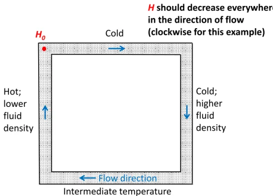
To evaluate the existence of hydraulic potentials in a variable-density system, consider the thought experiment for a thermally driven convection cell shown in Figure 3.
In this experiment, externally controlled temperature variations affect the fluid density (and viscosity) in each leg of the cell.
Figure 3 - Thermally driven convection cell. This figure illustrates a hypothetical closed loop consisting of a pipe filled with a saturated porous medium. The temperature in each leg of the cell can be externally controlled and maintained. In a laboratory setting, this might be accomplished using heating/cooling coils wrapped around each leg.
Cold
Cold;
higher fluid density
Intermediate temperature Hot;
lower fluid density
H
0H should decrease everywhere in the direction of flow
(clockwise for this example)
Flow direction
For this situation, experience indicates that density-driven flow will be induced in the pipe loop as shown. Our mission is to define a location-specific scaler quantity H that satisfies the rules for being a potential.
𝐻
0 is an arbitrary value assigned at the upper left corner of the pipe loop. To be a potential,𝐻
must decrease in the direction of flow and it must vary continuously with no jumps or discontinuities.Do you see the problem? If we assign a starting value of
𝐻
0 at the upper left corner and follow the flow path, it is possible for𝐻
to decrease in the direction of flow. However, as we come full circle and return to the starting location, the value of𝐻
would have to jump from a lower value to the higher starting value (𝐻
0). This would be a discontinuity, which cannot occur for a potential quantity. If𝐻
changes smoothly with no jumps, then somewhere in the system𝐻
would have to increase in the direction of flow, which also violates the rules for a potential.In fact, for this variable-density system, one cannot invent any scalar quantity that can be used in the head form of Darcy’s law to compute the correct flow direction at all locations. The head form of Darcy’s law might work for certain portions of this system, but it doesn’t work at all locations in the system. This is true no matter how you choose to define
𝐻
. The bottom line is that the head form of Darcy’s law cannot work for this variable-density system because no matter how one chooses to define head, it cannot exist as a hydraulic potential.Using energy considerations, M. K. Hubbert (1940, 1956) developed a complete definition of hydraulic head as shown in Equation (5).
𝐻(𝑧
′, 𝑃
′) = 𝛷
𝑔 = (𝑧′ − 𝑧
∗) + 1
𝑔 ∮ 1 𝜌(𝑃) 𝑑𝑃
𝑃′ 𝑃∗
(5) where (parameter dimensions are in dark green font with mass as M, length as L, time as T, temperature as Θ):
𝛷
= potential; work required to transform a unit mass of the fluid from an arbitrary reference state to the current state at a location of interest (L-2T-2)𝑧
∗ = arbitrary elevation of the reference state datum (L)𝑃
∗ = arbitrary pressure for the reference state (ML-1T-2)𝑧′
= elevation above the datum at the location of interest(L)𝑃
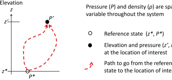
′ = pore fluid pressure at the location of interest (ML-1T-2)The small circle in the integral indicates that it is path independent, which implies that the integral has the same value regardless of the path taken in going from the reference state to the location of interest. Hubbert (1940, 1956) showed that for
𝐻
to exist as a potential, the integral must be path independent.Since the reference state is arbitrary, we can assign
𝑧
∗= 0 and𝑃
∗= 0. With these substitutions, Equation (5) simplifies to Equation (6).𝐻(𝑧
′, 𝑃
′) = 𝑧′ + 1
𝑔 ∮ 1 𝜌(𝑃) 𝑑𝑃
𝑃′ 0
(6) For the integral to be path independent, density must be a unique function of pressure. That means there can be no two points in the system where the pore water has the same pressure but different fluid densities. Otherwise, the integral is indeterminant and
𝐻
cannot exist as a potential quantity. This is illustrated in Figure 4.Figure 4 - Path from the reference state to the location of interest. In this system, pore water pressure and density both vary spatially. For hydraulic head to be a potential, the value of the integral in Equation (6) must be the same regardless of the path taken in going from 𝑃∗ to 𝑃′.
If the water density is everywhere constant,
𝜌
can come out of the integral in Equation (6) and the relationship simplifies to Equation (7), which is equivalent to the previously presented Equation (2):𝐻(𝑧
′, 𝑃
′) = 𝑧′ + 𝑃′
𝜌 𝑔
(7)However, this requires that the groundwater density (
𝜌
) is everywhere constant. We conclude that, from a theoretical perspective, the head form of Darcy’s law is strictly valid only in groundwater systems with spatially uniform fluid density.For variable-density groundwater flow systems, previous investigators have proposed different ways of defining head at a location of interest. For example,
ℎ
𝑓 in Equation (8) is referred to as the freshwater head, whileℎ
𝑝 in Equation (9) is referred to as pointwater head.ℎ
𝑓(𝑧
′, 𝑃′) = 𝑧
′+ 𝑃′
𝜌
𝑓𝑔
(8)z
Reference state (z*, P*)
Elevation and pressure (z’, P’) at the location of interest Path to go from the reference state to the location of interest z*
z’
P*
P’
Elevation
Pressure (P) and density (ρ) are spatially
variable throughout the system
ℎ
𝑝(𝑧
′, 𝑃
′)
=𝑧′ + 𝑃′
𝜌
′𝑔
(9)where:
𝑧′
= elevation at a specified location of interest (L)𝑃′
= pore water pressure at the location of interest (ML-1T-2)ℎ
𝑓 = freshwater head (L)𝜌
𝑓 = density of pure water at 20 °C (ML-3), which is 998.2 kg/m3ℎ
𝑝 = pointwater head (L)𝜌
′ = pore fluid density at the location of interest, that is, where𝑃′
is measured (ML-3)At this point, we define these proposed heads with a lowercase
ℎ
, as it has not been demonstrated that they are true hydraulic potentials that can work universally in the head form of Darcy’s law. We evaluate the applicability of these modified representations of head throughout this book.4 Pressure Form of Darcy’s Law
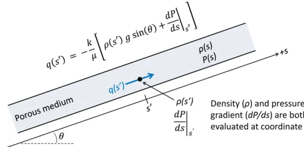
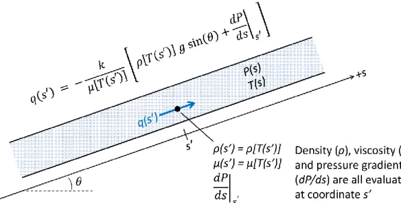
Referring to Figure 5, there is a second form of Darcy’s law that does not require use of a hydraulic potential. It is based on separate terms pertaining to gravity and pressure.
This is the pressure form of Darcy’s law shown in Equation (10).
𝑞(𝑠′) = − 𝑘
𝜇 [ 𝜌(𝑠
′) 𝑔 sin(𝜃) + 𝑑𝑃 𝑑𝑠 |
𝑠′
]
(10)where:
𝜃
= direction of flow from horizontal; counter-clockwise positive [radians or degrees]The other parameters were defined previously. In Equation 10 (and other subsequent equations), a combination of parentheses and brackets is used to better identify the computational grouping of terms.
Figure 5 - The one-dimensional pressure form of Darcy’s law. The derivative 𝑑𝑃 𝑑𝑠⁄ is the gradient of pressure evaluated at coordinate 𝑠’. Because there are two terms within the brackets, flow is not necessarily in the direction of decreasing pressure. Specific discharge (𝑞) is positive in the +𝑠 direction.
The specific discharge at coordinate
𝑠’, 𝑞(𝑠′)
, is the flow rate per unit cross-sectional area of the medium perpendicular to the𝑠
direction, the same as for the head form of Darcy’s law in Equation (1). The first term within the brackets is the𝑠-
direction component of the force per unit water volume due to gravity. The second term within the brackets is the𝑠-
direction component of the net force per unit water volume due to the pressure gradient (McWhorter & Sunada, 1977). Interestingly, when the𝑠
direction is horizontal (𝜃
is either 0 orπ
radians), there is no gravity effect and flow is driven solely by the pressure gradient in the direction of decreasing pressure. It has been said the head form of Darcy’s law sometimes works, but the pressure form of Darcy’s law always works. This is the version of Darcy’s law used in petroleum engineering.For an isotropic medium with a given pressure gradient (
𝑑𝑃 𝑑𝑠 ⁄
), this pressure form of Darcy’s law depends on the flow direction as defined by the angle𝜃
. For an anisotropic medium where intrinsic permeability (𝑘
) has directional properties, the pressure form of Darcy’s law becomes more complex with regard to gravity and pressure.4.1 Effect of Temperature
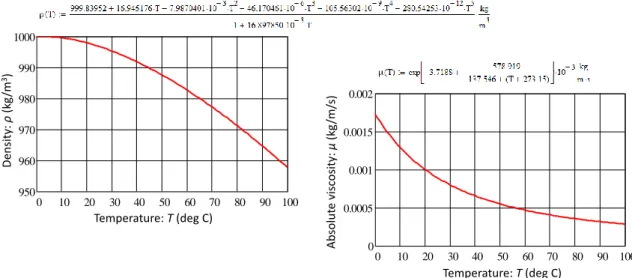
Let us first consider a low-salinity groundwater system with elevated temperatures, such as in a geothermal area. The density and viscosity of pure water change significantly with temperature. For example, when temperature increases from 20 to 80 °C:
• density of pure water decreases from 997.94 to 971.20 kg/m3 (a decrease of 2.68 percent), and
• viscosity decreases from 0.0010 to 0.00036 kg/m/s (i.e., lower by a factor of 2.82).
These variations are illustrated in Figure 6. Over this temperature range, the relative change in viscosity is much greater than the change in density.
Figure 6 - The effect of temperature on the density and dynamic viscosity of pure water at atmospheric pressure (i.e., zero gauge-pressure). T is temperature in °C. Above each graph is the empirical equation used to construct the curve. The empirical equation for water density is provided in Kell (1975). The empirical equation for viscosity is commonly referred to as the Vogel-Fulcher-Tamman equation or VFT equation, which is presented in CRC (2023).
If the temperature distribution along a one-dimensional flow path is known or estimated, the pressure form of Darcy’s law can be modified to:
𝑞(𝑠′) = − 𝑘
𝜇[𝑇(𝑠′)] [ 𝜌[𝑇(𝑠′)] 𝑔 𝑠𝑖𝑛(𝜃) + 𝑑𝑃 𝑑𝑠 |
𝑠′
]
(11)where (parameter dimensions are in dark green font with mass as M, length as L, time as T, temperature as Θ):
𝑇
= temperature (Θ) in °C for Celsius or °F for Fahrenheit𝑇(𝑠′)
= temperature (Θ) at coordinates’
as shown in Figure 7 (°C or °F)0 10 20 30 40 50 60 70 80 90 100 0
0.0005 0.001 0.0015 0.002
Temperature: T(deg C)
0 10 20 30 40 50 60 70 80 90 100 950
960 970 980 990 1000
Temperature: T(deg C)
Absolute viscosity: µ(kg/m/s)
Density: ρ(kg/m3)
Figure 7 - The pressure form of Darcy’s law for variable temperature. 𝑇(𝑠) is the temperature distribution along the 𝑠 direction. Groundwater density and dynamic viscosity are both functions of temperature as shown in Figure 6.
For a groundwater flow system with variable temperature, viscosity
𝜇[𝑇(𝑠)]
and density𝜌[𝑇(𝑠)]
can only have positive values. Inspection of Equation (11) shows that variations in viscosity can change the magnitude of specific discharge (𝑞
), but not the flow direction, and in variable temperature systems the effect on the magnitude of q can be very significant. In contrast, variations in density have the potential to change both the magnitude of q and the flow direction depending on whether the density change causes the summation within the brackets to change from positive to negative or vice versa.4.2 Effect of Salinity
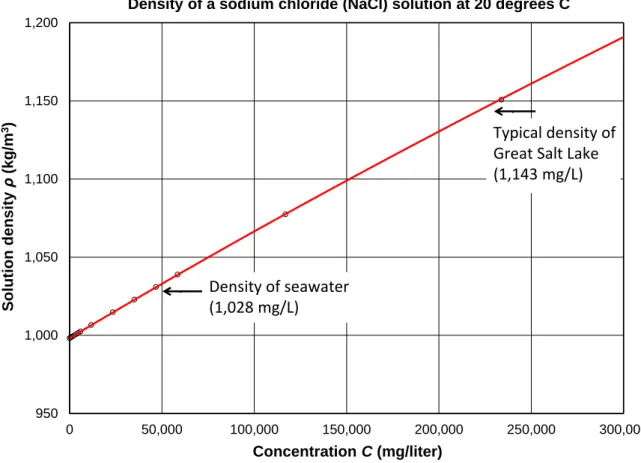
Now consider a groundwater system at atmospheric pressure (zero gauge-pressure) and a uniform temperature of 20 °C but with significant variations in salinity. The effect of salinity on groundwater density is complex and solute-specific. In general, the density of water increases with salinity, but there are some dissolved compounds for which the density decreases with increasing concentration in certain concentration ranges. Figure 8 shows the effect of a sodium chloride (
NaCl
) solution on water density. As can be seen, the effect is significant at high concentrations. In real systems, such high concentrations could occur at industrial/mining facilities, evapo-concentrated surface water bodies, deep connate groundwater brines associated with oil and gas development, and high-concentration groundwater contaminant plumes.Figure 8 - The effect of dissolved sodium chloride (NaCl) on water density. The system is at atmospheric pressure (zero gauge-pressure) and has a temperature of 20 °C. Relationships between water density and the concentrations of various dissolved solutes can be evaluated using the Drefahl (2023) online calculator.
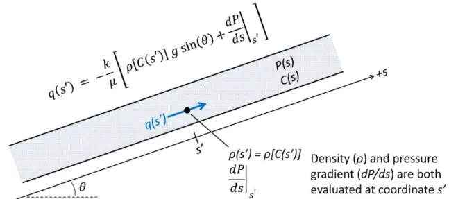
If the concentration distribution along a one-dimensional flow path is known or estimated, the pressure form of Darcy’s law can be modified as shown in Equation (12).
𝑞(𝑠′) = − 𝑘
𝜇 [ 𝜌[𝐶(𝑠′)] 𝑔 sin(𝜃) + 𝑑𝑃 𝑑𝑠 |
𝑠′
]
(12)where (parameter dimensions are in dark green font with mass as M, length as L, time as T, temperature as Θ):
𝐶
= solute concentration (ML-3)𝐶(𝑠)
= concentration (ML-3) along the𝑠
flow direction as shown in Figure 9950 1,000 1,050 1,100 1,150 1,200
0 50,000 100,000 150,000 200,000 250,000 300,000
Solution density ρ(kg/m3)
Concentration C (mg/liter)
Density of a sodium chloride (NaCl) solution at 20 degrees C
Density of seawater (1,028 mg/L)
Typical density of Great Salt Lake (1,143 mg/L)
Figure 9 - The pressure form of Darcy’s law for variable solute concentration. C(s) is the solute concentration distribution along the s direction. For sodium chloride (NaCl), the groundwater density as a function of concentration is shown in Figure 8.
4.3 Effect of Pressure
Water is a slightly compressible fluid. In going from 1 to 200 atm of pressure, the density of pure water at 20 °C increases from 998 to only 1,007 kg/m3; 200 atm of pressure is what would occur at the bottom of a static water column about 2,000 m high. For this reason, the effect of pressure on groundwater density is usually ignored in groundwater calculations. However, it could be important when evaluating very deep flow systems.
5 Solution of the Convection Cell Thought Experiment
Now let’s return to the thermally driven convection cell. For this thought experiment, we consider that the temperature in each leg of the pipe loop can be externally controlled using heating or cooling coils. Each leg of length L is maintained at a uniform temperature along its entire length. In the real world, if two legs have different temperatures, there would need to be a gradient (or transition) of temperature at the corner where the legs meet. Our thought experiment assumes that the temperature changes abruptly at each corner of the cell, which would not happen physically. However, for the issues being evaluated by this thought experiment, this departure from reality does not affect the conclusions reached.
The pipe loop is a closed system, that is, there is no addition of water or chemical mass from outside this system. The only thing that affects water density and viscosity is the externally imposed temperature in each leg. For steady-state flow, these conditions dictate that the mass flux of water in each leg must be the same. The mass flux (
𝑗
) is equal to the product of specific discharge times the fluid density (𝜌 𝑞
). Accordingly, we can multiply both sides of Equation (11) by density (𝜌
) to obtain the Mass Flux Equation (13).𝑗(𝑠′) = − 𝑘 𝜌[𝑇(𝑠′)]
𝜇[𝑇(𝑠′)] [ 𝜌[𝑇(𝑠′)] 𝑔 sin(𝜃) + 𝑑𝑃 𝑑𝑠 |
𝑠′
]
(13)where (parameter dimensions are in dark green font with mass as M, length as L, time as T, temperature as Θ):
𝑗
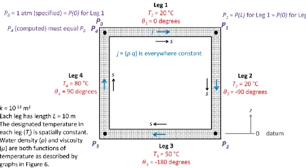
= mass flux (MT-1L-2)The setup for mathematical solution of the convection cell problem is shown in Figure 10. The cell contains four legs in a vertical plane, each of length L and with the same cross-sectional area. For our thought experiment, the mass flux (
𝑗
) is the same everywhere within the convection cell, and each leg has the temperature𝑇
𝑖where 𝑖 is the leg number 1, 2, 3, or 4.Figure 10 - Setup for solution of the convection cell thought experiment. P0 is an arbitrary fluid pressure assigned to the upper left corner of the cell. Each leg is assigned and index number 𝑖 = 1, 2, 3, 4 as shown.
Mass flux (j) is the same in each leg of the cell. P1, P2, P3, and P4 are computed pressures at the corners. P0 and P4 are the same point and therefore must have the same pressure.
For leg 𝑖 of the cell, the mass flux equation shown in Equation (14) applies (modified from Equation (13).
𝑗 = − 𝑘 𝜌[𝑇
𝑖]
𝜇[𝑇
𝑖] [ 𝜌[𝑇
𝑖] 𝑔 sin(𝜃
𝑖) + 𝑑𝑃 𝑑𝑠 |
𝑖
]
(14)where:
𝑇
𝑖 = uniform temperature along the length of leg𝑖
(Θ)Referring to Figure 10, the mass flux (
𝑗
) and temperature (𝑇
) are specified to be uniform, but different, within each leg, so the derivative of pressure (𝑑𝑃 𝑑𝑠 ⁄
) within a particular leg must also be uniform. The pressure gradient in leg i is therefore computed by Equation (15).𝑑𝑃 𝑑𝑠 |
𝑖
= 𝑃
𝑖(𝐿) − 𝑃
𝑖(0)
𝐿
(15)where:
𝑃
𝑖(0)
= water pressure at the upstream end of leg 𝑖 (ML-1T-2)𝑃
𝑖(𝐿)
= water pressure at the downstream end of leg 𝑖 (ML-1T-2)𝐿
= length of the convection cell leg (L)Substituting Equation (15) for the derivative in Equation (14) and solving for
𝑃
𝑖(𝐿)
leads to Equation (16) which applies to the conditions illustrated in Figure 11.𝑃
𝑖(𝐿) = 𝑃
𝑖(0) − 𝑗 𝐿 𝜇[𝑇
𝑖]
𝑘 𝜌[𝑇
𝑖] − 𝐿 𝜌[𝑇
𝑖] 𝑔 sin (𝜃
𝑖)
(16)Figure 11 - Pressure at each end of a convection cell leg. The entire leg has constant mass flux (j) and uniform temperature 𝑇𝑖.
For our convection cell, this formulation leads to a set of coupled equations shown in Equations (17) through (21).
Leg 1
𝑃
1= 𝑃
0− 𝑗 𝐿 𝜇[20
°𝐶]
𝑘 𝜌[20
°𝐶] − 𝐿 𝜌[20
°𝐶] 𝑔 sin(0 𝑑𝑒𝑔)
(17) Leg 2𝑃
2= 𝑃
1− 𝑗 𝐿 𝜇[20
°𝐶]
𝑘 𝜌[20
°𝐶] − 𝐿 𝜌[20
°𝐶] 𝑔 sin(−90 𝑑𝑒𝑔)
(18)Leg 3
𝑃
3= 𝑃
2− 𝑗 𝐿 𝜇[50
°𝐶]
𝑘 𝜌[50
°𝐶] − 𝐿 𝜌[50
°𝐶] 𝑔 sin(−180 𝑑𝑒𝑔)
(19) Leg 4𝑃
4= 𝑃
3− 𝑗 𝐿 𝜇[80
°𝐶]
𝑘 𝜌[80
°𝐶] − 𝐿 𝜌[80
°𝐶] 𝑔 sin(90 𝑑𝑒𝑔)
(20)𝑃
4= 𝑃
0 (21)To find a solution, Equations (17) through (20) are evaluated sequentially using an arbitrary
𝑃
0 in Equation (17) and a trial value for mass flux (𝑗
). Then, the computed𝑃
4 from Equation (20) is compared to the input𝑃
0. If they differ, a new mass flux value is tested.This process is repeated in a trial-and-error manner until a value of
𝑗
is found that results in Equation (21) being satisfied. When this is achieved, the associated𝑗
value is the uniform mass flux within the system being considered. In fluid mechanics, this iterative solution technique is known as the Hardy-Cross method. Armed with Equations (17) through (21), and the empirical relationships in Figure 6, we can now solve the convection cell problem shown in Figure 10 to obtain the system mass flux and the pressures at each corner of the convection cell. The calculations of pressure at each corner of the call are summarized in Table 1. With the solution obtained, we wish to further investigate the applicability of proposed alternate forms of hydraulic head within the system. Because the pressure gradient in each leg is linear, the pressure at the midpoint of a leg is equal to the average of the pressures at each end of the leg. Thus, at the midpoint of leg 𝑖, the freshwater head is given by Equation (22) and the pointwater head is given by Equation (23).ℎ
𝑓𝑚𝑖= 𝑧
𝑚𝑖+ 𝑃
𝑖−1+ 𝑃
𝑖2 𝑔 𝜌
𝑓 (22)ℎ
𝑝𝑚𝑖= 𝑧
𝑚𝑖+ 𝑃
𝑖−1+ 𝑃
𝑖2 𝑔 𝜌(𝑇
𝑖)
(23)where:
ℎ
𝑓𝑚𝑖 = freshwater head at the midpoint of convection cell leg 𝑖 (L)𝑧
𝑚𝑖 = midpoint elevation of convection cell leg 𝑖 (L)ℎ
𝑝𝑚𝑖=
pointwater head at the midpoint of convection cell leg i (L)Calculations of freshwater head and pointwater head are summarized in Table 1, and the results are shown graphically in Figure 12.
Table 1 - Calculations for the convection cell thought experiment. To provide detailed documentation, these calculations are performed using MathCad® software. However, the equations could also be evaluated using a calculator or spreadsheet. The MathCad® output contains a semicolon before the equal sign and a dot to indicate multiplication of parameters and units (MathCad® treats units as parameters).
Figure 12 - Results of the convection cell thought experiment. In portions of the cell, the fluid flow is in the direction of increasing freshwater head (hf) and/or increasing pointwater head (hp), indicating that these parameters are not true hydraulic potentials.
For this thought experiment, the mathematical results show that freshwater head (
ℎ
𝑓) and pointwater head (ℎ
𝑝) are not hydraulic potentials because in some portions of the cell the flow is in the direction of increasing values. As such, it is somewhat misleading to describe these parameters as heads and interpret them as alternate representations of the parameter𝐻
used in the head form of Darcy’s law. Blindly replacing𝐻
withℎ
𝑓 orℎ
𝑝 in Equation (1) would not provide the true flow directions or magnitudes at all locations within the cell. For this variable-density flow system, the hydraulics can only be solved using the pressure form of Darcy’s law. The bottom line is that the hydraulic potential𝐻
is a different “animal” fromℎ
𝑓 orℎ
𝑝 because the latter are not true hydraulic potentials.Further, the downward flow in the right leg of the cell in Figure 12 is in the direction of increasing pressure, so pressure alone is not a true potential for describing flow.
In Figure 12, an interesting observation is that specific discharge increases slightly where the cell attains higher temperature. One might ask: Why does the specific discharge change if there are no sources or sinks that add or subtract flow to/from the system? For this closed flow system, conservation of mass implies that the mass flux (
𝑗 = 𝜌𝑞
) is everywhere constant. If the fluid density𝜌
decreases (at higher temperature), the specific discharge𝑞
must increase. This can also be explained by thermal expansion of the fluid at higher temperature.6 Application of Darcy’s Law to Groundwater Systems
Having shown that the head form of Darcy’s law did not work for our convection cell thought experiment, there is some good news for groundwater hydrologists. In most natural groundwater systems, the difference in groundwater density is sufficiently small that its variation can be ignored, and calculations can proceed using a uniform (average) density. When this assumption is justified, the hydraulic head form of Darcy’s law can be used, and the errors imposed are not large enough to be of practical concern. This explains why the hydraulic head form of Darcy’s law is embedded in the thinking of the groundwater discipline: It usually works! However, there are situations where one may need to use the pressure form of Darcy’s law to obtain more representative results.
Examples include the following:
• in a freshwater aquifer, the horizontal migration of a groundwater chemical plume with very high TDS;
• vertical groundwater flow in an aquitard that is sandwiched between two aquifers, one with relatively fresh water and one with brine, a situation known to occur adjacent to Great Salt Lake in Utah, USA;
• deep groundwater flow in a geothermal area;
• vertical upward flow of lower TDS groundwater toward shallow higher TDS groundwater associated with a playa lake;
• groundwater flow passing over the top of a salt dome;
• along coastlines where a freshwater aquifer is in hydraulic contact with an aquifer containing ocean water; and
• where high-concentration chemical reagents are injected into groundwater for in situ treatment.
A practical approach for groundwater professionals can be to perform scoping-level, one-dimensional flow solutions using both the head and pressure forms of Darcy’s law and compare the results. If the results are very similar, one can usually proceed with the head form using a uniform (average) fluid density and have a reasonable expectation that the results will be sufficiently accurate for practical application. If results of the two forms of Darcy’s law are significantly different, deferral to the pressure form may be required to obtain defensible results. For example, if both equations give the same flow direction but a magnitude difference less than, say, 10 percent, one might conclude that the uncertainty of the results is small compared to the uncertainty in the value of
𝑘
(or 𝐾), and either method is adequate for practical application. However, if the two methods give different flow directions, the pressure form of Darcy’s law should take precedent.The relative effect of temperature (
𝑇
) on water viscosity (𝜇) is always greater than its effect on water density (𝜌
). At face value, one might conclude that the temperature effecton viscosity could swamp the effect on density. However, the system hydraulics may be more complicated than this simple interpretation. The flux equation presented previously for a system with zero solute concentration—but with elevated/variable temperature as shown in Equation (11)—is reproduced here as Equation (24).
𝑞(𝑠′) = − 𝑘
𝜇 [𝑇(𝑠′)] [𝜌[𝑇(𝑠′)] 𝑔 sin(𝜃) + 𝑑𝑃 𝑑𝑠 |
𝑠′
]
(24)This equation shows that the magnitude of flux (
𝑞
) is inversely proportional to viscosity, and this effect can be significant. However, a change in viscosity alone does not affect the flow direction. The direction of flow is controlled by the term[𝜌[𝑇(𝑠)] 𝑔 sin(𝜃) +
𝑑𝑃 𝑑𝑠⁄ |
𝑠′]
. If this term is negative, flow is in the +𝑠
direction; if positive, flow is in the −𝑠
direction. Therefore, in a variable temperature system, one cannot necessarily neglect the magnitude/variation in groundwater density even though the relative variation in viscosity is much greater.The flux equation presented as Equation (12) for a system at standard temperature, but with an elevated/variable solute concentration, is reproduced here as Equation (25).
𝑞(𝑠′) = − 𝑘
𝜇 [ 𝜌[𝐶(𝑠′)] 𝑔 sin(𝜃) + 𝑑𝑃 𝑑𝑠 |
𝑠′
]
(25)Except for extreme cases of certain organic compounds (such as biodegradable slurries), we can usually ignore the effect of concentration on water viscosity.
Elevated/variable concentration can significantly change the groundwater density, and this can affect both flow direction and magnitude as expressed by the bracketed term.
7 Horizontal Flow Calculations
Let’s consider some practical situations. The first is essentially horizontal flow in an aquifer where the groundwater density varies laterally but not vertically. If the principal directions of hydraulic conductivity are horizontal and vertical, we can relax the isotropic assumption and consider horizontal hydraulic conductivity (
𝐾
ℎ) or horizontal intrinsic permeability (𝑘
ℎ) in calculations of horizontal flow.For horizontal flow, the direction angle (𝜃) is zero and the pressure form of Darcy’s law shown by Equation (10) simplifies to Equation (26) where the coordinate direction x is used to indicate that the flow direction is horizontal.
𝑞
ℎ(𝑥′) = − 𝑘
ℎ𝜇
𝑑𝑃 𝑑𝑥 |
𝑥′
(26) where (parameter dimensions are in dark green font with mass as M, length as L, time as T, temperature as Θ):
𝑞
ℎ = horizontal specific discharge (LT-1)𝑘
ℎ = horizontal intrinsic permeability (L2)𝑥
′ = specified horizontal coordinate (L)Horizontal flow is controlled only by the gradient of pressure. Conveniently, the density of the groundwater in the aquifer and its spatial variation ρ(s) falls out of the flow equation.
Let’s evaluate the horizontal component of flow in an aquifer between two monitoring wells. To proceed, we must select an arbitrary horizontal reference level at elevation
𝑧
𝑟 and estimate the fluid pressure (𝑃
𝑟) at each well at that elevation as shown in Figure 13. Replacing the derivative in Equation (26) with a finite difference approximation, an estimate of the horizontal specific discharge is given by Equation (27) where an approximation sign is used because a linear hydraulic gradient is assumed between𝑥
1and𝑥
2.𝑞
ℎ≈ − 𝑘
ℎ𝜇
(𝑃
𝑟2− 𝑃
𝑟1)
(𝑥
2− 𝑥
1)
(27)where:
𝑃
𝑟𝑖 = pressure at the reference elevation at the location of well i (ML-1T-2)𝑥
𝑖 = distance coordinate at the location of well𝑖
(L)Figure 13 - Estimation of horizontal specific discharge in an aquifer with variable-density groundwater. The magnitude/variation of groundwater density between the wells is not needed to perform the calculation. The equation for
𝑞
ℎhas an approximation sign because a linear pressure gradient is assumed to exist between the wells.7.1 Estimation of Pressure at the Reference Elevation
Equation (27) is easy to solve. However, a practical challenge is estimating the fluid pressures
𝑃
𝑟1 and𝑃
𝑟2 at the chosen reference elevation (𝑧
𝑟). As shown in Figure 14, we typically install a groundwater monitoring well and measure the physical water-level elevation in the well or fluid pressure at the elevation of a pressure transducer installed somewhere within the water column.Figure 14 - Typical groundwater monitoring well installation. Parameters shown on the figure are described in the text.
Reference level
Well 1 Well 2
Pr1 Pr2
x1 x2 x
qh
ρ z
tP
wElevation
z , h
z
rReference level
ρ Ground
P
rWell
P
atmh
wTransducer: P
tgor P
taz
wThe parameters represented in Figure 14 are as follows. Parameter dimensions are in dark green font with mass as M, length as L, time as T, temperature as Θ.
𝑧
𝑤 = midpoint elevation of well completion zone (L)𝑧
𝑟 = reference level elevation (L)𝑧
𝑡 = pressure transducer elevation (L)ℎ
𝑤 = physical water-level elevation in a well (L)𝜌
= groundwater density in the vicinity of the well (ML-3)𝑃
𝑤 = fluid pressure at the midpoint of a well completion zone (ML-1T-2)𝑃
𝑟 = groundwater pressure at the reference level (ML-1T-2)𝑃
𝑎𝑡𝑚 = prevailing atmospheric pressure (ML-1T-2)𝑃
𝑡𝑔 = gauge pressure measured by a vented submersible transducer (ML-1T-2)𝑃
𝑡𝑎 = absolute pressure measured by an unvented submersible transducer (ML-1T-2)We assume that the monitoring well is periodically purged, so the density of the water column in the casing is the same as groundwater in the aquifer (
𝜌
). Using well measurements, we compute the groundwater pressure at the reference level (𝑃
𝑟) at the well location making the following assumptions.• The vertical pressure distribution in the aquifer is hydrostatic (no upward or downward flow).
• The vertical pressure distribution in the well-water column is hydrostatic.
•
𝑃
𝑤 is the fluid pressure in the well-completion zone and in the adjacent geologic formation at elevation𝑧
𝑤.• The groundwater density (
𝜌
) is vertically uniform at the well location.• The average density of the well-water column is the same as the groundwater density (
𝜌
).These assumptions are reasonable for many groundwater situations. The assumptions say the vertical pressure distribution inside the well is the same as the vertical pressure distribution in the adjacent aquifer.
Hydraulic conditions in a monitoring well or piezometer can be evaluated by measuring any of the following.
• The distance from a surveyed measuring point (typically the top of the well casing) down to the physical water level in the well. This is usually done using an electric depth-to-water tape that indicates when its bottom probe contacts the water surface. Subtracting this distance from the elevation of the measuring point gives the elevation of the water surface (
ℎ
𝑤).• Measurement of gauge pressure (
𝑃
𝑡𝑔) using a vented pressure transducer that does not require a barometric correction. For this type of instrument, the readout pressure is zero when sensing the atmosphere regardless of the prevailing barometric pressure.• Measurement of absolute pressure (
𝑃
𝑡𝑎) by a submersible pressure transducer positioned at a known elevation in the water column. Referred to as an unvented pressure transducer, when this instrument senses the atmosphere at sea level, its readout pressure is approximately 100,300 pascals (Pa) or 14.7 pounds per square inch (psi). To convert absolute pressure to gauge pressure requires a correction using the prevailing barometric pressure, which is typically measured using an external barometer at ground surface or accessing barometric records from a nearby weather station.Other measurement devices are available,