It can be used to offer various types of data mining courses with different emphases. He served as the Vice President of the SIAM Activity Group on Data Mining.
Introduction
For example, a commercial product recommendation problem is very different from an intrusion detection application, even at the input data format or problem definition level. For example, a product recommendation problem in a multidimensional database is very different from a social recommendation problem because of the differences in the underlying data type.
The Data Mining Process
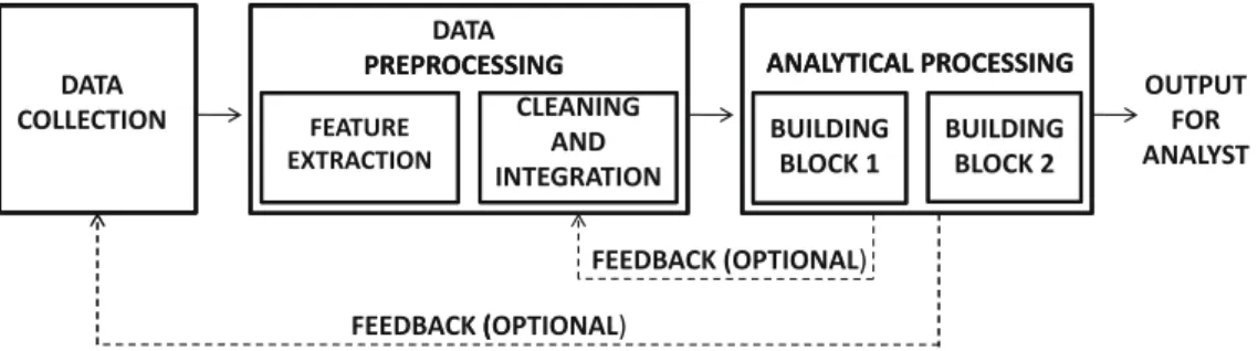
Note that the analytical block in Fig. 1.1 shows several building blocks that represent the design of the solution for a particular application. The second is the demographic information in the retailer database that was collected during web registration of the customer.
THE DATA MINING PROCESS 5 of any use to the retailer. In the feature extraction process, the retailer decides to create
The Data Preprocessing Phase
Feature selection and transformation should not be considered part of data preprocessing because the feature selection stage is often highly dependent on the specific analytical problem being solved. However, the feature selection phase is usually performed before the specific algorithm in question is applied.
The Analytical Phase
AN INTRODUCTION TO DATA MINING The data cleaning process requires statistical methods commonly used for missing data estimation. In some cases, the feature selection process may even be tightly integrated with the specific algorithm or methodology used, in the form of a wrapper model or embedded model.
The Basic Data Types
THE BASIC DATA TYPES 7 Table 1.1: An example of a multidimensional data set
Nondependency-Oriented Data
This is called binary data and can be considered as a special case of numerical or categorical data. In practice, a vector space representation is used, where the frequencies of the words in the document are used for analysis.
THE BASIC DATA TYPES 9 algorithm is often unlikely to work with sparse data without appropriate modifications
Dependency-Oriented Data
An important aspect of time series mining is the extraction of such dependencies in the data. As in the case of time series data, the contextual attribute is a timestamp or a position index in the sequence.
THE BASIC DATA TYPES 11 It should be noted that the aforementioned definition is almost identical to the time-
In a meteorological application, Xi may contain temperature and pressure attributes at location Li. In such cases, temperature is a behavioral attribute, while spatial and temporal attributes are contextual.
THE BASIC DATA TYPES 13
Network data is a very general representation and can be used to solve many similarity-based applications on other data types. It is possible to use community detection algorithms to determine clusters in the network data and then map them back to multidimensional data.
The Major Building Blocks: A Bird’s Eye View
For example, multidimensional data can be transformed into network data by creating a node for each record in the database and representing the similarity between the nodes with edges. MAIN BUILDINGS: A BIRD'S VIEW 15 when the entries in a row are very different from the corresponding entries in others.
THE MAJOR BUILDING BLOCKS: A BIRD’S EYE VIEW 15 when the entries in a row are very different from the corresponding entries in other
Association Pattern Mining
The confidence of the rule A ⇒ B is defined as the fraction of transactions containing A that also contain B. In other words, the confidence is obtained by dividing the support of the pattern A∪B by the support of pattern A.
Data Clustering
Nevertheless, this particular definition of association pattern mining has become the most popular one in the literature due to the ease of developing algorithms for it. In fact, many variations of the association pattern mining problem are used as a subroutine to solve the clustering, outlier analysis, and classification problems.
THE MAJOR BUILDING BLOCKS: A BIRD’S EYE VIEW 17 An important part of the clustering process is the design of an appropriate similarity
Outlier Detection
Event detection is one of the primary motivating applications in the field of sensor networks. Identifying fraud in financial transactions, trading activities or insurance claims typically requires determining unusual patterns in the data generated by the actions of the criminal entity.
Data Classification
Compared to other major data mining problems, the classification problem is relatively self-contained. On the other hand, the classification problem is often used directly as a stand-alone tool in many applications.
Impact of Complex Data Types on Problem Definitions
Hence, from a learning perspective, clustering is often referred to as unsupervised learning (due to the lack of a specific training database to "teach" the model about the notion of appropriate clustering), while the classification problem is referred to as supervised learning. The classification problem is related to association pattern mining, in the sense that the latter problem is often used to solve the former.
Scalability Issues and the Streaming Scenario
In such cases, the volume of the data is so large that it may be impractical to store directly. The amount of data that can be processed at a given time depends on the storage available to hold segments of the data.
A Stroll Through Some Application Scenarios
Store Product Placement
For example, the pattern of sales in a given hour of a day may not be similar to that at another hour of the day. It is often challenging to design algorithms for such scenarios because of the variable rate at which the patterns in the data can change over time and the constantly evolving patterns in the underlying data.
A STROLL THROUGH SOME APPLICATION SCENARIOS 23
Customer Recommendations
Medical Diagnosis
AN INTRODUCTION TO DATA MINING if previous examples of normal and abnormal series exist. Furthermore, the class labels are likely to be unbalanced because the number of abnormal series is usually much smaller than the number of normal series.
Web Log Anomalies
Summary
BIBLIOGRAPHIC NOTES 25
Bibliographic Notes
Exercises
Which data mining problem would be suitable for the task of identifying groups among the remaining customers who might buy widgets in the future. Which data mining problem would be best suited to find sets of items that are frequently purchased together with widgets.
Introduction
Data reduction, selection and transformation: In this phase, the size of the data is reduced by means of data subset selection, feature subset selection or data transformation. First, when the size of the data is reduced, the algorithms are generally more efficient.
Feature Extraction and Portability
Feature Extraction
Data cleaning: The data cleaning phase removes missing, erroneous, and inconsistent entries from the data. Second, removing irrelevant attributes or irrelevant records improves the quality of the data mining process.
FEATURE EXTRACTION AND PORTABILITY 29 popular. This is a semantically rich representation that is similar to document data
Data Type Portability
One challenge with discretization is that the data cannot be uniformly distributed over the different intervals. Thus, using ranges of equal size may not be very useful for distinguishing between different data segments.
FEATURE EXTRACTION AND PORTABILITY 31 Table 2.1: Portability of different data types
Value-based discretization: The (already averaged) values of the time series are discretized into a smaller number of approximately equi-depth intervals. Interval bounds are constructed by assuming that the time series values are distributed with a Gaussian assumption.
FEATURE EXTRACTION AND PORTABILITY 33 2.6 Discrete Sequence to Numeric Data
Note that the similarity graph can be sharply defined for data objects of any type, as long as an appropriate distance function can be defined. This is why distance function design is so important for virtually any data type.
Data Cleaning
Note that this approach is only useful for applications based on the concept of similarity or distances. DATA CLEANING 35. The above problems can be a significant source of inaccuracy for data mining applications.
DATA CLEANING 35 The aforementioned issues may be a significant source of inaccuracy for data mining appli-
Handling Missing Entries
For example, in a time series data set, the mean of the values at the time stamp just before or after the missing feature can be used for estimation. For the case of spatial data, the estimation process is quite similar, where the mean values at neighboring spatial locations can be used.
Handling Incorrect and Inconsistent Entries
In the case of dependency-oriented data, such as time series or spatial data, estimating missing values is much simpler. Alternatively, behavioral values in the last n time series data stamps can be linearly interpolated to determine the missing value.
Scaling and Normalization
Data Reduction and Transformation
Sampling
In the unbiased sampling method, a predetermined fraction f of data points is selected and retained for analysis. Thus, no duplicates are included in the sample unless the original data set also contains duplicates.
DATA REDUCTION AND TRANSFORMATION 39 δt time units ago, is proportional to an exponential decay function value regulated by
Feature Subset Selection
Unsupervised features: This corresponds to removing noisy and redundant features from the data. Therefore, a discussion of unsupervised feature selection methods is deferred to Chapter 6 on data clustering.
DATA REDUCTION AND TRANSFORMATION 41
Dimensionality Reduction with Axis Rotation
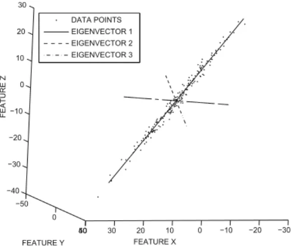
PCA is usually applied after subtracting the mean of the data set from each data point. Thus, the (i, j)th entry of C indicates the covariance between the ith and jth columns (dimensions) of the data matrix D.
DATA REDUCTION AND TRANSFORMATION 43 An interesting property of this diagonalization is that both the eigenvectors and eigenval-
However, these distinct methods are sometimes confused with each other because of their close relationship. Note that the diagonal matrix Σ is rectangular and not square, but it is called diagonal because only the entries of.
DATA REDUCTION AND TRANSFORMATION 45 form Σ ii are nonzero. It is a fundamental fact of linear algebra that such a decomposition
Note that the total energy in the data set D is always equal to the sum of the squares of all nonzero singular values. 3 The squared error is the sum of the squares of the entries in the error matrix D−QkΣkPkT.
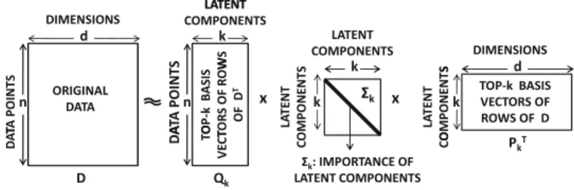
DATA REDUCTION AND TRANSFORMATION 47 The orthonormal columns of Q k provide a k-dimensional basis system for (approximately)
Dimensionality Reduction with Type Transformation
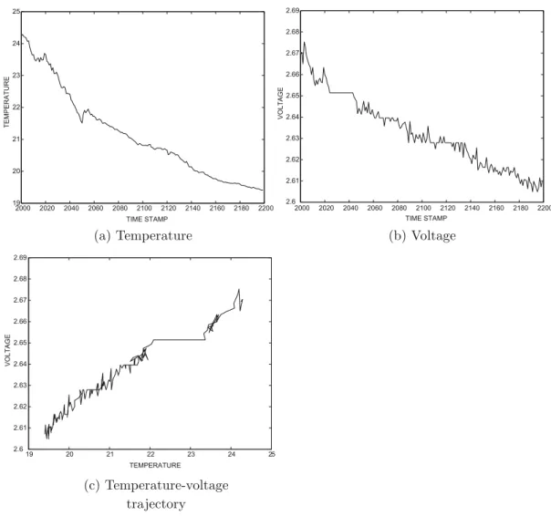
It gives an idea of the temperature, but not much more about the variation over the day. This process can be applied recursively down to the granularity level of the sensor readings.
DATA REDUCTION AND TRANSFORMATION 51
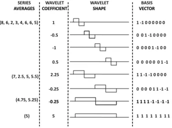
The number of wavelet coefficients in this series is 8, which is also the length of the original series. The number of wavelet coefficients (and basis vectors) is equal to the length of the string.
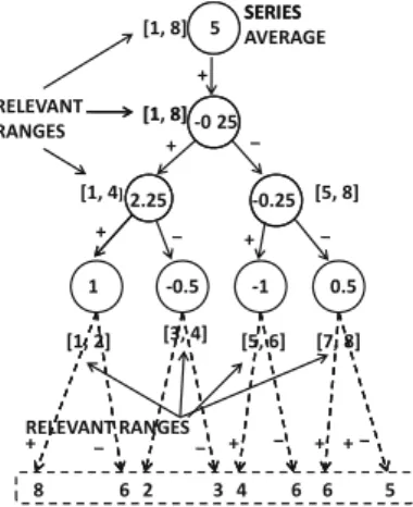
DATA REDUCTION AND TRANSFORMATION 53 The length of the time series representing each basis vector is also q. Each basis vector has
DATA REDUCTION AND TRANSFORMATION 53The length of the time series representing each basis vector is alsoq. In this section, a brief overview of the extension of wavelets to several contextual attributes is given.
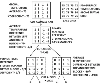
DATA REDUCTION AND TRANSFORMATION 55 by successive divisions. These divisions are alternately performed along the different axes
Note that SVD also derives the optimal embedding as the scaled eigenvectors of the dot product matrix of the original data. It is desirable to embed the nodes of this graph in ak-dimensional space so that the similarity structure of the data is preserved.
Summary
The data set may be very large, and it may be desirable to reduce its size in terms of both the number of rows and the number of dimensions. To reduce the number of columns in the data, feature subset selection or data transformation can be used.
Bibliographic Notes
These methods are closely related to analytical methods because the importance of properties can depend on the application. In the first row, the axis system can be rotated to match the correlations of the data and retain the directions of maximum variance.
Exercises
Treat each quantitative variable in the KDD CUP 1999 Network Intrusion Data Set from the UCI Machine Learning Repository[213] as a time series. Create samples of size n records from the data set from the previous exercise and determine the mean value ei of each quantitative column i using the sample.
Introduction
Some data types, such as multidimensional data, are much easier to define and calculate distance functions than with others, such as time series data. In some cases, user intents (or training feedback on object pairs) are available to oversee the design of the distance feature.
Multidimensional Data
Quantitative Data
2, spectral embedding can be used to transform a similarity graph built on any type of data into multidimensional data. Although this chapter focuses primarily on unsupervised methods, we will also briefly touch on the broader principles of using supervised methods.
MULTIDIMENSIONAL DATA 65
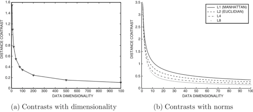
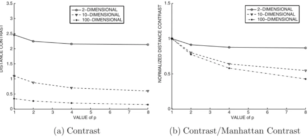
Indeed, this behavior is observed for all Lp-norms at different values of p, albeit with varying severity. On the other hand, a different set of characteristics will be more important for a group containing patients with epilepsy.
MULTIDIMENSIONAL DATA 67
A broader principle that seems to work well for high-dimensional data is that the impact of the noisy variation along individual attributes should be attenuated while the cumulative match is counted across many dimensions. Therefore, an approach that can automatically adapt to the dimensionality of the data is needed.
MULTIDIMENSIONAL DATA 69
The Mahalanobis distance is similar to the Euclidean distance except that it normalizes the data based on the inter-attribute correlations. The Mahalanobis distance is equal to the Euclidean distance in such a transformed (axes-rotated) data set after dividing each of the transformed coordinate values by the standard deviation of the data in that direction.
MULTIDIMENSIONAL DATA 71
Categorical Data
In the context of categorical data, the aggregated statistical properties of the dataset should be used when calculating similarity. As in the case of the inverse frequency of occurrence, a higher match value is assigned to a match when the value is infrequent.
Mixed Quantitative and Categorical Data
Text Similarity Measures
Measures such as the Lp rate do not adapt well to the varying lengths of different documents in the collection. The cosine measure calculates the angle between two documents, which is insensitive to the absolute length of the document. yd) be two documents in a lexicon of size
TEMPORAL SIMILARITY MEASURES 77
Binary and Set Data
Temporal Similarity Measures
Time-Series Similarity Measures
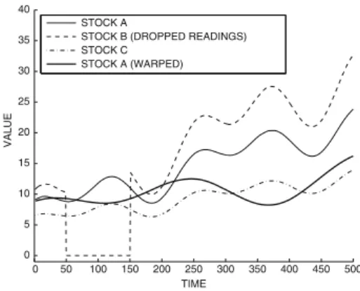
In such cases, the value of the time attribute should be shifted in at least one of the time series to allow more efficient matching. An additional complication is that different time segments of the string may need to be convoluted differently to allow a better match.
TEMPORAL SIMILARITY MEASURES 79
Within the distance Lp there is a one-to-one mapping between the timestamps of the two time series. This can be used to artificially create two strings of the same length that have a one-to-one mapping between them.
TEMPORAL SIMILARITY MEASURES 81
Discrete Sequence Similarity Measures
Discrete sequence similarity measures are based on the same general principles as time series similarity measures. As with time series data, discrete sequential data may or may not have a one-to-one mapping between positions.
TEMPORAL SIMILARITY MEASURES 83 transform one string to another with a sequence of insertions, deletions, and replacements
The goal here is to either match the last element of Xi and Yj, or remove the last element in one of the two sequences. In such a case, the last element of at least one of the two strings must be removed on the assumption that it cannot appear in the matching.
GRAPH SIMILARITY MEASURES 85
Graph Similarity Measures
Similarity between Two Nodes in a Single Graph
The structure measure from the previous section does not work well when pairs of nodes have different number of paths between them. The random walk measure therefore provides a result that is different from the result of the shortest path measure because it also considers the multiplicity of paths during the similarity calculation.
Similarity Between Two Graphs
In random walk-based similarity, the approach is as follows: Imagine a random walk starting at source nodes and continuing to a neighboring node with weighted probability proportional to wij. You are more likely to reach a location that is close by and can be reached in multiple ways.
Supervised Similarity Functions
This objective function can be optimized with respect to Θ using any off-the-shelf optimization solver. Using a closed form such as f(Oi, Oj,Θ) ensures that the function f(Oi, Oj,Θ) can be efficiently computed at the one-time cost of computing the parameters Θ.
Summary
The problem of learning remote features can be modeled more generally as that of classification. Supervised remote function design using Fisher's method is also discussed in detail in the instance-based learning section in Chap.10.
Bibliographic Notes
The relationship between the maximal ordinary subgraph problem and the graph modification distance problem is studied in [119,120]. The problem of distance feature learning has been formally linked to that of classification and has recently been studied in great detail.
Exercises
Suppose the insertion and deletion costs are 1 and the replacement cost is 2 units per edit distance. Show that the optimal edit distance between two strings can be computed using only insertion and deletion operations.
Introduction
The frequency model for association pattern mining is very popular because of its simplicity. Therefore, many models have been proposed for frequent pattern mining based on statistical significance.
The Frequent Pattern Mining Model
Other Important Data Mining Problems: Frequent pattern mining can be used as a subroutine to provide effective solutions to many data mining problems such as clustering, classification, and outlier analysis. Because the frequent pattern mining problem was originally proposed in the context of market basket data, a significant amount of terminology used to describe both the data (e.g., transactions) and outputs (e.g., item sets) is borrowed from the supermarket analogy.
THE FREQUENT PATTERN MINING MODEL 95 Table 4.1: Example of a snapshot of a market basket data set
Therefore, an appropriate choice of support level is essential for detecting a set of frequent patterns of significant size. In the example of Table 4.1, the set of items{Egg, milk, Yoghurt} is a set of frequent items at a minimum support level of 0.3.
ASSOCIATION RULE GENERATION FRAMEWORK 97
Association Rule Generation Framework
The first phase is more computationally intensive and therefore the most interesting part of the process. Therefore, the discussion of the first phase will be deferred to the remainder of this chapter, and a brief discussion of the (simpler) second phase is given here.
Frequent Itemset Mining Algorithms
Brute Force Algorithms
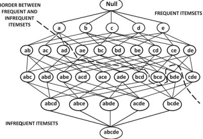
Reduce the size of the explored search space (grid of Figure 4-1) by pruning candidate item sets (grid nodes) using tricks such as the downclosure property. The first algorithm to make use of effective search space pruning using the downward closing property was the Apriorial algorithm.
The Apriori Algorithm
ASSOCIATION PATTERN MINING regular pattern mining searches the grid of possibilities (or candidates) for regular patterns (see Fig.4.1) and uses the transaction database to count the support of candidates in this grid. To count the support of each candidate more efficiently by trimming transactions known to be irrelevant to counting a candidate itemset.
FREQUENT ITEMSET MINING ALGORITHMS 101 Algorithm Apriori(Transactions: T , Minimum Support: minsup)
A leaf node of the hash tree contains a list of lexicographically sorted topic sets, whereas an internal node contains a hash table. Assume that the root of the hash tree is level 1 and that all subsequent levels below it increment by 1.
FREQUENT ITEMSET MINING ALGORITHMS 103
Enumeration-Tree Algorithms
However, only the former is possible in the enumeration tree after the lexicographic order has been fixed. Most of the counting tree algorithms work by growing this counting tree of frequent itemsets with a predefined strategy.
FREQUENT ITEMSET MINING ALGORITHMS 105 Algorithm GenericEnumerationTree(Transactions: T ,
TreeProjection is a family of methods that use recursive projections of transactions onto the enumeration tree structure. The special case T(N ull) = T corresponds to the highest level of the enumeration tree and is equivalent to the complete transaction database.
FREQUENT ITEMSET MINING ALGORITHMS 107 Algorithm ProjectedEnumerationTree(Transactions: T ,
The strategy used to select the node P determines the order in which the nodes of the enumeration tree materialize. In this case, only the databases projected along the current enumeration tree path being explored need to be maintained.
FREQUENT ITEMSET MINING ALGORITHMS 109 of transactions. Of course, this process only provides transaction counts and not itemset
In a depth-first strategy, it can be shown that a pattern of length 20 will be discovered after exploring only 19 of its immediate prefixes. Further intersection of the resulting label list with that of the second item gives support for the 3-item.
FREQUENT ITEMSET MINING ALGORITHMS 111 Table 4.2: Vertical representation of market basket data set
Recursive Suffix-Based Pattern Growth Methods
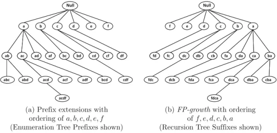
This relationship between recursive pattern growth methods and numbered tree methods will be explored in more detail in Section 4.4.4.5. COMMON SUFFIX MINING ALGORITHMS 113 Recursive suffix-based pattern growth methods are generally understood in context.
FREQUENT ITEMSET MINING ALGORITHMS 113 Recursive suffix-based pattern growth methods are generally understood in the context
The projected set of transactions Ti will become smaller at deeper levels of recursion in terms of number of items and number of transactions. An alternative is to output all the Ti and T projections corresponding to the various suffix items simultaneously in a single database scan just before the for loop is initiated.
FREQUENT ITEMSET MINING ALGORITHMS 115
The path from the root to the leaf of the trie represents a (possibly repeated) transaction in the database. Each internal node is associated with a count representing the number of transactions in the original database that contain the prefix corresponding to the path from the root to that node.
FREQUENT ITEMSET MINING ALGORITHMS 117
Again, this conditional FP tree is a sample representation of the conditional pointer base in Fig. For example, in the case of FIG. 4.11, all nodes on the conditional FP tree lie on a single path.
FREQUENT ITEMSET MINING ALGORITHMS 119 Algorithm FP-growth(FP-Tree of frequent items: FPT , Minimum Support: minsup,
Traditional enumeration tree methods typically count the support of a single layer of rare extensions of the frequent patterns in the enumeration tree as (failed) candidates to exclude them. This is because the enumeration tree is a sub-graph of the grid (candidate space) and it provides a way to explore the candidate patterns in a systematic and non-redundant way.
Alternative Models: Interesting Patterns
Accounting for sets of designed transactions can be done in different ways using different data structures, such as arrays, pointers, or a pointer-proof combination. Many different variations of the data structure have been explored in different projection algorithms, such as TreeProjection, DepthProject, FP-growth and H-Mine[419].
ALTERNATIVE MODELS: INTERESTING PATTERNS 123 Although it is possible to quantify the affinity of sets of items in ways that are statisti-
- Statistical Coefficient of Correlation
- χ 2 Measure
- Interest Ratio
- Symmetric Confidence Measures
Symmetric confidence measures can be used to replace the support-confidence framework with a single measure. Symmetric confidence measures can be derived as a function of X ⇒Y confidence and Y ⇒X confidence.
ALTERNATIVE MODELS: INTERESTING PATTERNS 125
- Cosine Coefficient on Columns
- Jaccard Coefficient and the Min-hash Trick
- Collective Strength
- Relationship to Negative Pattern Mining
Any off-the-shelf frequent pattern mining algorithm can be applied to this binary matrix to discover relevant combinations of columns and identifiers. The advantage of the off-the-shelf approach is that there are many efficient algorithms available for the common pattern mining model.
Useful Meta-algorithms
Sampling Methods
False positives: These are patterns that meet the support threshold in the sample, but not in the base data. False negatives: These are patterns that do not meet the support threshold in the sample, but meet the threshold in the data.
Data Partitioned Ensembles
Many depth-first algorithms on the summary tree can be challenged by these scenarios because they require random access to the transactions. Reducing the support thresholds too much will lead to many spurious itemsets and increase the work in the post-processing phase.
SUMMARY 129
Generalization to Other Data Types
Summary
ASSOCIATION PATTERN MINING The Apriori algorithm is one of the earliest and best known methods for regular pattern mining. A number of sampling methods have been designed to improve the efficiency of regular pattern mining.
Bibliographic Notes
Association rules can be determined in quantitative and categorical data using type transformations. BIBLIOGRAPHICAL NOTES 131Eclatpaper [537] reveals that this is a memory optimization of the breadth-first approach by.
BIBLIOGRAPHIC NOTES 131 Eclat paper [537] reveals that it is a memory optimization of the breadth-first approach by
Exercises
Construct a prefix-based FP tree for the lexicographic ordering a, b, c, d, e, f for the data set in Exercise 1. Construct a prefix-based FP tree for the lexicographic ordering a, b, c, d , e, f for the data set in Exercise 5.
Introduction
ASSOCIATION PATTERN MINING: ADVANCED CONCEPTS Table 5.1: Example of a snapshot of a market basket data set (Repeated from Table 4.1 in Chap.4). A query-friendly compression schema is very different from a summary schema designed to ensure non-redundancy.
Pattern Summarization
Maximal Patterns
However, the shrinking of the discovered topic sets is due to the constraints rather than a compression or summarization scheme. PATTERN SUMMARIZATION 137 Although all itemsets can be derived from the maximal itemsets with the subsetting.
PATTERN SUMMARIZATION 137 Although all the itemsets can be derived from the maximal itemsets with the subsetting
Closed Patterns
Each item set in S(X) describes the same set of transactions, and therefore it is sufficient to keep the single representative item set. The maximum itemsetX from S(X) is retained. The set of frequent itemsets at a given minimum support level can be determined and the closed frequent itemsets can be derived from this set.
PATTERN SUMMARIZATION 139 by the current or a previous traversal. After the traversal is complete, the next unmarked
Approximate Frequent Patterns
To achieve this goal, the subset of the itemset grid representing F can be traversed in the same way as discussed in the previous case of (exactly) closed sets. The idea of the greedy algorithm is to start with J ={} and add the first element from F to J that covers the maximum number of itemsets in F .
Pattern Querying
Preprocess-once Query-many Paradigm
In the preprocess-enquery-many-query paradigm, itemsets are mined at the lowest possible support level so that a large frequent part of the itemsets network (graph) can be stored in main memory. The network has a number of important properties, such as downward closure, that allow the discovery of non-redundant association rules and patterns.
PATTERN QUERYING 143
The actual item sets indexed by each signature table entry are stored on disk. Each entry in the signature table references a list of pages containing the sets of items indexed by that supercoordinate.
PATTERN QUERYING 145
Pushing Constraints into Pattern Mining
However, in practice, the constraints can be much more general and cannot be easily handled by any particular data structure. In such cases, constraints may need to be pushed directly into the mining process.
Putting Associations to Work: Applications
Relationship to Other Data Mining Problems
Because association patterns determine highly correlated subsets of attributes, they can be applied to quantitative data after discretization to identify dense regions in the data. Nevertheless, the resulting clusters correspond to dense regions in the data that provide important insight into the underlying clusters.
Market Basket Analysis
Intuitively, the set of elements X is discriminative between the two classes if the absolute difference in the confidence of the rules X ⇒c1 and X ⇒c2 is as large as possible. A transaction is said to be covered by an association pattern when the corresponding association pattern is contained in the transaction.
Demographic and Profile Analysis
Interestingly, even a relatively simple modification of the association framework to the classification problem was discovered to be quite efficient. This approach is particularly useful in scenarios where the data is high-dimensional and traditional distance-based algorithms cannot be easily used.
PUTTING ASSOCIATIONS TO WORK: APPLICATIONS 149 rules are very useful for target marketing decisions because they can be used to identify
- Recommendations and Collaborative Filtering
- Web Log Analysis
- Bioinformatics
- Other Applications for Complex Data Types
Frequent pattern mining algorithms have been generalized to more complex data types such as temporal data, spatial data, and graph data. The analysis of the frequent patterns in the call graphs and key deviations from these patterns provides insight about the errors in the underlying software.
Summary
Spatial co-location patterns: Spatial co-location patterns provide useful insights about the spatial relationships between different individuals. Chemical and biological graph applications: In many real-world scenarios, such as chemical and biological compounds, the determination of structural patterns provides insight into the properties of these molecules.
Bibliographic Notes
ASSOCIATION PATTERN MINING: ADVANCED CONCEPTS of regular pattern mining methods for graph applications, such as software error analysis, and chemical and biological data, are provided in Aggarwal and Wang [26].
Exercises
Introduction
In this chapter and the next, the study of clustering will be limited to simpler multidimensional data types, such as numeric or discrete data. More complex data types, such as temporary or network data, will be studied in later chapters.
Feature Selection for Clustering
Filter Models
In filter models, a specific criterion is used to evaluate the impact of specific features, or subsets of features, on the clustering tendency of the data set. In such domains, it makes more sense to talk about the presence or absence of non-zero values on the attributes (words), rather than distances.
FEATURE SELECTION FOR CLUSTERING 157 a systematic way to search for the appropriate combination of features, in addition to
Wrapper Models
Since the search space of feature subsets is exponentially related to dimensionality, a greedy algorithm can be used to successively drop features, resulting in the largest improvement in the cluster validity measure. Use any controlled measure to quantify the quality of individual properties against L-marks.
Representative-Based Algorithms
CLUSTER ANALYSIS In other words, the sum of the distances of the various data points from their closest representatives should be minimized. Note that the assignment of data points to representatives depends on the choice of representativesY1.
REPRESENTATIVE-BASED ALGORITHMS 161
The k-Means Algorithm
In the thek-means algorithm, the sum of the squares of the Euclidean distances of data points to their nearest representatives is used to quantify the objective function of the clustering. In such a case, it can be shown1 that the optimal representative Yj for each of the "optimal" iterative steps is the mean of the data points in the cluster Cj.
REPRESENTATIVE-BASED ALGORITHMS 163
The Kernel k-Means Algorithm
The k-Medians Algorithm
The k-Medoids Algorithm
REPRESENTATIVE ALGORITHMS 165 selected from the database D, and this difference requires changes in the underlying structure.
REPRESENTATIVE-BASED ALGORITHMS 165 selected from the database D , and this difference necessitates changes to the basic structure
CLUSTER ANALYSIS for initialization criteria, choice of number of clusters k and presence of outliers. The simplest initialization criteria are either to randomly select points from the domain of the data space, or to sample the original database D.
Hierarchical Clustering Algorithms
Because these centroids are more representative of the database D, this provides a better starting point for the algorithm. This will result in splitting some of the data clusters into multiple representatives, but it is less likely that clusters will be merged incorrectly.
HIERARCHICAL CLUSTERING ALGORITHMS 167
Bottom-Up Agglomerative Methods
This clustering will require the distance matrix to be updated to a smaller (nt-1)×(nt-1) matrix. The advantage of the latter criterion is that it can be intuitively interpreted according to the number of groups in the data.
HIERARCHICAL CLUSTERING ALGORITHMS 169
Accordingly, the matrix M in this case is updated using the maximum values of the rows (columns). Variance-based criterion: This criterion minimizes the change in the target function (such as cluster variance) due to merging.
HIERARCHICAL CLUSTERING ALGORITHMS 171
Top-Down Divisive Methods
The overall approach for top-down clustering uses a general-purpose flat-clustering algorithm as a subroutine. In each iteration, the data set at a specific node of the current tree is divided into multiple nodes (clusters).
Probabilistic Model-Based Algorithms
After the parameters of the mixture components have been estimated, the posterior generative (or assignment) probabilities of data points with respect to each mixture component (cluster) can be determined. A striking observation is that if the probabilities of data points generated from different clusters were known, it becomes relatively easy to determine the optimal model parameters separately for each component of the mixture.
PROBABILISTIC MODEL-BASED ALGORITHMS 175 corresponding to random assignments of data points to mixture components), and proceeds
Relationship of EM to k-means and Other Representative MethodsMethods