This part of the book explores the general properties of algorithms and defines various notions of convergence. Each part of the book contains enough material to form the basis of a quarter course.
Introduction
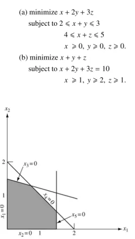
- Optimization
- Types of Problems
- Size of Problems
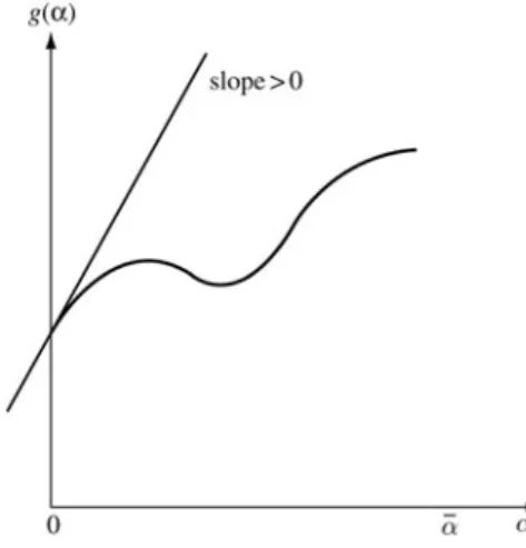
- Iterative Algorithms and Convergence
Of course, the theoretical and computational aspects assume a somewhat special character for linear programming problems - the most important development being the simplex method. This issue was finally resolved when it was found that it was possible for the number of steps to be exponential in the size of the program.
Linear Programming
Basic Properties of Linear Programs
- Introduction
- Examples of Linear Programming Problems
- Basic Solutions
- The Fundamental Theorem of Linear Programming
- Relations to Convexity
- Exercises
If we substitute u1−v1zax1 everywhere in (2.1), the linearity of the constraints is preserved and now all variables must be non-negative. Note that the matrix of coefficients can be divided into blocks corresponding to variables of different time periods.
The Simplex Method
Pivots
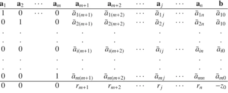
Denoting the coefficients of the new system in canonical form by ¯aij, we have explicitly. In particular, the expression forbin terms of the base is given in the last column.
Adjacent Extreme Points
The coefficients of the other vectors will either increase or decrease linearly as they increase. If none of the ¯aiqs are positive, then all coefficients in the representation (3.16) increase (or remain constant) as they increase, and no new fundamentally feasible solution is obtained.
Determining a Minimum Feasible Solution
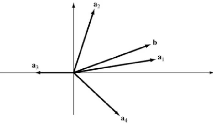
In the figure, a basic feasible solution can be constructed with positive weights on and2 because there is between them. Optimality Condition Theorem. If for a fundamentally feasible solution cj−zj0for all j, then that solution is optimal.
Computational Procedure: Simplex Method
Some further discussion of the relative cost coefficients and the bottom line of the table is warranted. We notice that the objective function—we are using the negative of the original one—.
Finding a Basic Feasible Solution
If (3.27) is solved using the simplex technique, we get a basic feasible solution at each step. There is no obvious basic feasible solution to this problem, so we introduce artificial variables x6 and x7.
Matrix Form of the Simplex Method
The revised simplex method is a scheme for ordering the calculations required of the simplex method so that unnecessary calculations are avoided. The revised form of the simplex method is as follows: Given the inverseB−1 of a current basis, and the current solutionxB=a¯0=B−1b,. One can go a step further in the matrix interpretation of the simplex method and note that the execution of a single simplex cycle is not explicitly dependent on B−1, but rather on the ability to solve linear systems with Bas the coefficient matrix.
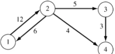
Simplex Method for Transportation Problems
This means that the first step of the procedure for verifying triangularity is satisfied. The triangularity of the basis guarantees that this procedure can be carried out to determine all the simplex multipliers. The cost coefficients of the problem are shown in the array below, with the circled cells corresponding to the current basic variables.
3.8 Decomposition
Summary
As the value of this variable increases, the values of the current basis variables are continuously adjusted so that the total vector continues to satisfy the system of linear equality constraints. At this point, the value of one of the basic variables is zero and that variable is declared non-basic, while the non-basic variable that was incremented is declared basic. The most important property of the transportation problem is that any basis is triangular.
Exercises
Show that if there is a fundamentally feasible solution (possibly degenerate) for the unperturbed system with baseB = [a1, a2, . Show that corresponding to any fundamentally feasible solution to the perturbed system of Exercise15, which is non-degenerate for a range of ε > 0, and with a vector node in the basis, there is a unique vector j in the basis which, when replaced by ak , leads to a fundamentally feasible solution ; and that solution is non-degenerate for a range of ε >0. Suppose the phase I procedure is applied to systemAx=b, x0, and the resulting tableau (ignoring the cost row) has the form.
Letz0 denotes the current value of the objective function at a stage of the simplex algorithm, (cj−zj) the corresponding relative cost coefficients, and. Assuming this problem is solved by the simplex method and it is sufficient to obtain a solution within tolerance from the optimal value of the objective function, specify a stopping criterion for the algorithm in terms of and the parameters of the problem. Without loss of generality, we assume that the current basis consists of the last mcolumns.
Duality and Complementarity
- Dual Linear Programs
- The Duality Theorem
- Relations to the Simplex Procedure
- Sensitivity and Complementary Slackness
- Max Flow–Min Cut Theorem
- The Dual Simplex Method
The vector xis the variable of the primal program, andy is the variable of the dual program. The dual of any linear program can be found by converting the program to the form of the primitive form above. The duality relations can be viewed in terms of the dual interpretations of linear constraints emphasized in Chapter 3.
4.7 ∗ The Primal-Dual Algorithm
Summary
Exercises
Show that Xis guaranteed a wage of at least no matter what is chosen by Y. b) Show that the dual of the above problem is the minimization of B. Hint: Use the dual simplex method.) Plotλ2(f) and net profit (f) excluding cost for cotton. Show that in the bounded bounded dual of the primal-dual method the objectiveTb can be replaced by ngayTy.
Interior-Point Methods
Elements of Complexity Theory
For the algorithms we consider in this chapter, the obvious choice is the set of the four arithmetic operations and the comparison. Examples of the first are fixed-precision floating-point numbers stored in a fixed amount of memory (usually 32 or 64 bits). Examples of the second are integers, which require a number of bits approximately equal to the logarithm of their absolute value.
5.2 ∗ The Simplex Method Is Not Polynomial-Time
When comparing algorithms, it should be made clear which computational model is used to derive the limits of complexity. A problem can be solved in polynomial time if a polynomial time algorithm exists that solves the problem. The concept of polynomial time is usually understood as the formalization of efficiency in complexity theory.
5.3 ∗ The Ellipsoid Method
The Analytic Center
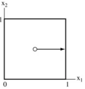
The analytic center S is the vector (or set of vectors) that minimizes the potential; it is the vector (or vectors) that solve. Therefore, the analytic center is identical to what would normally be called the center of the unit cube. The analytic center of Ω is the interior point of Ω that minimizes the potential function.
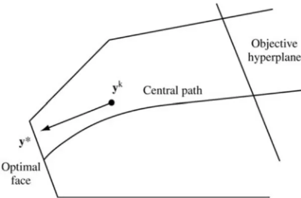
The Central Path
Therefore, the central path in this case is a straight line that progresses from the analytic center of the square (atμ→ ∞) to the analytic center of the optimal face (atμ→0). To see the geometrical representation of the central dual path, consider the dual level set. Then, the analytic center (y(z), s(z)) of Ω(z) coincides with the central dual path ascending to the optimal value∗from below.
Solution Strategies
The idea of the path-following method is to move within a tubular neighborhood of the central path towards the solution point. The step ≡ (dx, dy, ds) is defined by the linearized version of the central primal-dual path equations of (5.9), as. Therefore, the dual primal-potential function gives a clear limit on the size of the duality gap.
Termination and Initialization
The fifth approach is to guess the optimal surface and project the current interior point onto the interior of the optimal surface. A practically significant drawback of this approach is the doubled dimension of the system of equations that must be solved at each iteration. A linear program is called self-dual if the dual of the problem is equivalent to the primal.
Summary
It does not require regularity assumptions regarding the existence of optimal, feasible, or internally feasible solutions. It can be initialized at x = 1, y = 0 etc = 1, feasible or infeasible, on the central ray of the positive ortans (cone), and it does not require a large-Constraint parameter or lower bound. If the linear program has a solution, the algorithm generates a sequence that approaches feasibility and optimality simultaneously; if the problem is infeasible or unbounded, the algorithm produces an infeasibility certificate for at least one of the primal and dual problems; see Exercise 5.
Exercises
Much of this material is based on Cottle's teaching note on linear programming, which he taught at Stanford [C6]. The central pathway was analyzed in McLinden [M3], Megiddo [M4] and Bayer and Lagarias [B3,B4], Gill et al. A more practical predictor-corrector algorithm was proposed by Mehrotra [M5] (see also Lustig et al. [L19] and Zhang and Zhang [Z3]).
Conic Linear Programming
Convex Cones
When k=1 they become dimensional vectors and the inner product is the standard dot product of two vectors. In SDP, this definition is almost always used for the case where the matrices are both square and symmetric. It is not difficult to see that the two cones in the first two cones in Example 1 are all themselves; while the dual cone of the p-order cone is the q-order cone where.
Conic Linear Programming Problem
For simplicity, assuming ZS DP>0, it has been shown that in many cases of this problem an optimal SDP solution either constitutes an exact solution or can be rounded to a good approximate solution of the original problem. In the former case, one can show that a rank-1 optimal solution matrix Y exists for the semi-definite relaxation and it can be found using a rank reduction procedure. In this way, one can find a feasible solution to the original problem whose objective value is not less than a factor α of the true maximum objective cost.
Farkas’ Lemma for Conic Linear Programming
But if the distance measurements are noisy, one can add additional variables and add an error target to minimize it. Under a given graph structure, an optimal SDP solution of the formulation would be guaranteed to be an exact solution to the original problem. We would like to prove that for every double cone (including the cone of the second order) the point (v;y) holds.
Conic Linear Programming Duality
Constraint (6.9) is of the form appearing in the dual form of a semidefinite program. Again, the matrix restriction is of the double form of a semidefinite cone, but its dimension is fixed at 2. But this is only the other side of the proof given that Fd is feasible and has a feasible solution of interior, dhez∗ is also the supreme of (KLD).
Complementarity and Solution Rank of SDP
Again, let X∗ be an optimal SDP solution with rank>d and we factorizeX∗as. One can further show that ˆX would be a good approximate solution of the SDP in many cases. One can further show ˆx would be a good approximate solution to the original binary QP.
Interior-Point Algorithms for Conic Linear Programming
Note that X0 and S0 do not need to satisfy other equality constraints, so they can be easily identified. The optimal objective value of (HSDCLP) is zero, that is, any optimal solution of (HSDCLP) has. The question is: how is an optimal solution of (HSDCLP) related to optimal solutions of original (CLP) and (CLD).
Summary
We are now ready to apply the interior point algorithm, starting with the available initial feasible interior point solution, to solve (HSDCLP).
Exercises
In Lovasz and Shrijver [159] a "lifting" procedure is proposed to get a problem in n2; and then the problem is projected back to obtain stricter inequalities; see also Balas et al. An overscaling (potential reduction) algorithm for semi-definite programming is due to Alizadeh [A4,A3] where Yinyu Ye "suggested to study the over-potential function for this problem" and "to symmetric preserving scalings of the formX0 −1/ to look" 2XX−1/20 ”, and to Nesterov and Nemirovskii [N2]. The homogeneous and self-dual initialization model was originally developed by Ye, Todd, and Mizuno for LP [Y2], and for SDP by de Klerk et al.
Unconstrained Problems
Basic Properties of Solutions and Algorithms
- First-Order Necessary Conditions
- Examples of Unconstrained Problems
- Second-Order Conditions
- Convex and Concave Functions
7.2 (a) Power Requirement Curve; (b)x1 and x2 indicate the capacities of the nuclear power stations and the coal-fired power stations respectively. The proof of Theorem 1 in Section 7.1 is based on making a first-order approximation of the function f near the relative minimum point. Theorem 2 (Second Order Necessary Conditions – Unrestricted Case). Let x∗ be an internal point of the setΩ, and suppose that x∗ is a relative minimum point overΩ of the function f∈C2. 7.6) For simplicity of notation, we often denote ∇2f( x), then ×nmatrix of the second partial derivative of f, the Hessian of f, by the alternative notation F(x).