Deciphering regulation in Escherichia coli: from genes to genomes

(1)

to genomes

Thesis by

Suzannah Michelle Beeler

In Partial Fulfillment of the Requirements for the Degree of

Doctor of Philosophy in Biology

CALIFORNIA INSTITUTE OF TECHNOLOGY Pasadena, California

2022

Defended July 22, 2021

(2)

Suzannah Michelle Beeler ORCID: 0000-0002-1930-4827

Some rights reserved. This thesis is distributed under a Creative Commons Attribution License CC-BY 4.0.

(3)

ACKNOWLEDGEMENTS

First and foremost I must thank my PhD advisor, Rob Phillips. I have learned so much from him during the time I’ve spent with him in the lab and in the classroom.

He has instilled in me the immense value of biological numeracy and the ability to tackle problems in biology from pure thought alone. I can safely say that my PhD was far from typical, but in a way that has prepared me for my next steps better than I could have ever imagined. With Rob I have been given the opportunity to teach at the Marine Biological Laboratory, at GIST in Korea, and even in New Zealand and the Galápagos with the Caltech Alumni. With these innumerable teaching experiences, I eagerly await the next stage of my academic career where I intend to spread the immeasurable value of a quantitative understanding of biology to my future students.

Within the realm of teaching quantitative biology, Justin Bois has also been an immense source of inspiration. Within my first years at Caltech, I had the pleasure of taking four classes from him, imbuing me with skills that I used throughout the remainder of my graduate career. And while I only had the opportunity to TA with him once, I will remain inspired by his thoughtful and rigorous approach to teaching. When explaining my future job as a teaching faculty member to my current colleagues, numerous people have responded with “so you’ll be their version of Justin?" and I aspire to be even half as influential as he has been here at Caltech.

Throughout my time in the lab, I have seen many fellow graduate students come and go. Regardless of the precise make-up of the lab, the Phillips lab has always been marked by its strong collaborative spirit and I have rarely had to work alone.

Specifically, when I first joined the lab, I was graciously guided by Stephanie Barnes, Nathan Belliveau, and Bill Ireland as I was ushered into the Sort-Seq part of the group. Though a daunting task, Bill and I worked together for many years to bring the Sort-Seq approach into the new era of Reg-Seq. With this new era came a new set of people working on the regulatory genome of E. coli: Tom Röschinger and Scott Saunders have recently joined the lab and Manuel Razo-Mejia has switched gears slightly from his in-depth dissections of thelacoperon to more genome-wide approaches, through the use of RNA-Seq. I have deeply enjoyed my time with them all as the “socialists,” and while I am the first of our group to leave Caltech, I can’t wait to see where our project ends up, even if it is from afar.

(4)

Other members of the lab, though I have not had the opportunity to work with them directly, have also been a source of immeasurable support. Griffin Chure has been an friend, ally, and font of knowledge throughout my time in lab. He is an inspiration not just as a scientist, but also as a human being. While we hardly spoke back when I was first rotating in the lab, I’m glad I’ve gotten to know Soichi Hirokawa better through our adventures to Woods Hole, New Zealand, and Korea.

He helped me face some truly harrowing situations including the Tokyo subway system and a night with far too much soju. Lastly, the following members of the lab have been a source of support over the years, whether as administrators, office mates, or company on coffee breaks: Pamela Albertson, Rachel Banks, Celene Barrera, Kimberly Berry, Adam Catching, Ana Duarte, Tal Einav, Avi Flamholz, Helen Bermudez Foley, Vahe Galstyan, Jonathan Gross, Zofii Kaczmarek, Heun Jin Lee, Gita Mahmoudabadi, Niko McCarty, Muir Morrison, Rebecca Rousseau, Gabe Salmon, and Franz Weinert.

Outside of the lab, there are numerous people who have supported me. Primarily, the self proclaimed ‘Broads of Broad’: Grace Chow, Annisa Dea, Sarah Gillespie, Heidi Klumpe, Christina Su, Lynn Yi, and Shinae Yoon. They have all been a source of inspiration and served to make my time as a woman at Caltech less isolating.

Outside of Caltech, Misha Vysotskiy has been my best friend throughout grad school and well before. We’ve faced every academic stage together, starting with taking CS70 together at Harvey Mudd College in 2012. From there, we were Mathematical and Computational Biology majors, faced the graduation school application process, and even traveled to some interviews together. And we’re still standing after all this time.

On a personal side, I want to thank those who have been with me long before my time at Caltech began: my parents. Whether helping me learn to read with flashcards, testing me on my spelling words on the way to school, or looking over my math homework, they have always been committed to me and my academic success. Their endless sacrifice made sure I endured even through a childhood riddled with illness and other hiccups. I’m incredibly privileged and lucky to have ‘made it’, and I know it would not have been possible without their commitment to me.

Lastly, I am so incredibly grateful to have spent the last 8+ years with my partner Tobin Ivy, and look forward to many, many more. During our time at Caltech, he has evolved from my boyfriend to my roommate to my fiancé. I can’t wait to start the next chapter of our lives, building a life and a home together in Colorado.

(5)

ABSTRACT

Advances in DNA sequencing have revolutionized our ability to read genomes.

However, even in the most well-studied of organisms, the bacterium Escherichia coli, for ≈ 65% of promoters we remain ignorant of their regulation. Until we crack this regulatory Rosetta Stone, efforts to read and write genomes will remain haphazard. We introduce a new method, Reg-Seq, that links massively-parallel reporter assays with mass spectrometry to produce a base pair resolution dissection of more than 100E. colipromoters in 12 growth conditions. We demonstrate that the method recapitulates known regulatory information. Then, we examine regulatory architectures for more than 80 promoters which previously had no known regulatory information. In many cases, we also identify which transcription factors mediate their regulation. This method clears a path for highly multiplexed investigations of the regulatory genome of model organisms, with the potential of moving to an array of microbes of ecological and medical relevance.

(6)

PUBLISHED CONTENT AND CONTRIBUTIONS

Ireland, W. T., S. M. Beeler, E. Flores-Bautista, N. S. McCarty, T. Röschinger, N. M.

Belliveau, M. J. Sweredoski, A. Moradian, J. B. Kinney, and R. Phillips (2020).

“Deciphering the regulatory genome of Escherichia coli, one hundred promoters at a time”. In: eLife. issn: 2050084X. doi: 10 . 7554 / eLife . 55308. eprint:

2001.07396.

S.M.B helped design, optimize, and conduct experiments, and helped write and create figures for the manuscript.

(7)

LIST OF ILLUSTRATIONS

Number Page

1.1 Examples of diauxic growth. . . 2

1.2 Regulation of thelacoperon. . . 4

1.3 Microstates of RNA polymerase binding to DNA. . . 6

1.4 Pictorial representation of 𝑝_bound. . . 7

1.5 States and weights for polymerase binding. . . 8

1.6 States and weights for simple repression. . . 9

1.7 Theory meets experiment for simple repression. . . 10

1.8 Regulatory ignorance across the domains of life. . . 11

1.9 Evidence of gene regulation in un-annotated genes. . . 12

1.10 The Sort-Seq protocol. . . 13

1.11 Expression shift for the mutagenizedlacpromoter. . . 14

1.12 An example of mutual information on a piece of text. . . 16

1.13 An example of mutual information between DNA sequence and gene expression. . . 18

1.14 All regulatory architectures uncovered in this thesis. . . 19

2.1 TheE. coliregulatory genome. . . 26

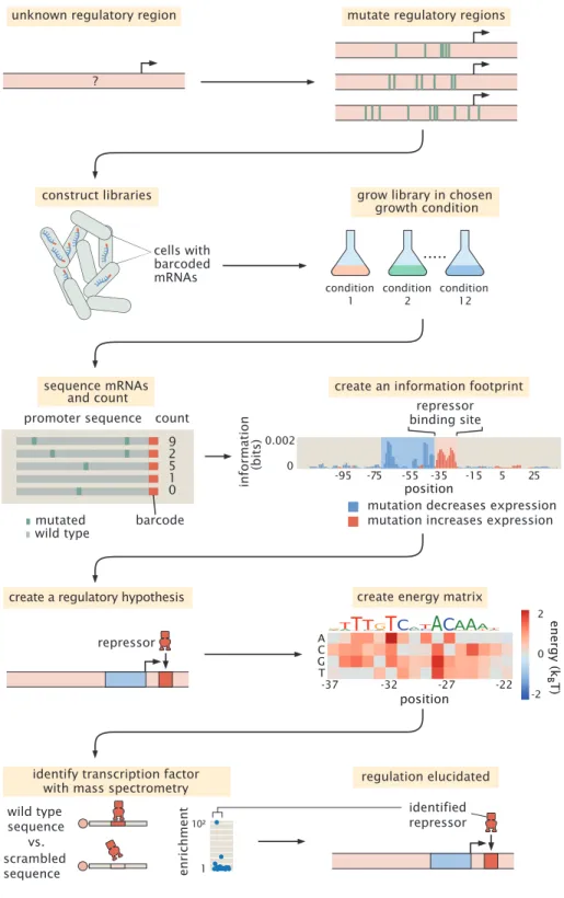
2.2 Schematic of the Reg-Seq procedure as used to recover a repressor binding site. . . 27

2.3 A summary of four direct comparisons of measurements from Sort- Seq and Reg-Seq. . . 29

2.4 All regulatory architectures uncovered in this study. . . 34

2.5 Examples of the insight gained by Reg-Seq in the context of promoters with no previously known regulatory information. . . 36

2.6 A summary of regulatory architectures discovered in this study. . . . 38

2.7 GlpR as a widely-acting regulator. . . 47

2.8 FNR as a global regulator. . . 48

2.9 Inspection of a genetic circuit. . . 49

2.10 Representative view of the interactive figure that is available online. . 50

2.11 Procedure to identify binding site regions automatically. . . 60

2.12 Schematic of the genetic construct used in this study. . . 62

2.13 Mock data comparing Sort-Seq and Reg-Seq sequence logo values. . 67

(9)

2.14 A visual comparison of the literature binding sites and the extent of

the binding sites discovered by our algorithmic approach. . . 75

2.15 A visual display of the results of the TOMTOM motif comparison between the discovered binding sites and known sequence motifs from RegulonDB and our prior Sort-Seq experiment . . . 76

2.16 Pearson correlation as a function of the number of unique DNA sequences. . . 85

2.17 Motif comparison using TOMTOM for the two PhoP binding sites in theybjXpromoter. . . 94

2.18 Two cases in which we see transcription factor binding sites that we have found to regulate both of the two divergently transcribed genes. . 95

2.19 A comparison of the types of architectures found in RegulonDB to the architectures with newly discovered binding sites found in the Reg-Seq study. . . 97

3.1 Theory meets experiment for simple repression. . . 112

3.2 Barcode coverage for the three wildtype operator sequences. . . 113

3.3 Operator coverage of the O1 library. . . 114

(10)

LIST OF TABLES

Number Page

2.1 All promoters examined in this study, categorized according to type of regulatory architecture. . . 39 2.2 All genes investigated in this study categorized according to their

regulatory architecture . . . 45 2.3 All growth conditions used in the Reg-Seq study. . . 65 2.4 A suite of experimentally validated and high-evidence binding sites

used to test our automated binding site finding algorithm. . . 69 2.5 The results of the comparison between experimentally verified, high

evidence binding sites and Reg-Seq binding sites. . . 71 2.6 Example dataset of 4 nucleotide sequences, and the corresponding

counts from the plasmid library and mRNAs. . . 77 2.7 Global, absolute quantification for most transcription factors identi-

fied in this study. . . 86 2.8 Example energy matrix. . . 89 2.9 Example dataset with energy predictions. . . 90 2.10 Scaling factors to convert arbitrary units to absolute units in 𝑘_𝐵𝑇. . . 92 2.11 Key Resource Table. . . 110

(11)

C h a p t e r 1

INTRODUCTION: ON A QUANTITATIVE UNDERSTANDING OF GENE REGULATION

1.1 Introduction

Adaptation is nearly synonymous with being alive. The commonly used adage ‘life finds a way’ hints at the universality of adaptation within the living world. The concept of adaptation should be familiar from our day-to-day lives. As an example, our eyes are able to adjust from broad daylight to a dark room in a matter of minutes through the dilation of our pupils, permitting more light to enter our eyes. In this way, we adapt to our environment in a way that makes it more suitable for our survival. It should come as no surprise that adaptation such as this occurs across all domains of life, although the exact mechanism of adaptation may be qualitatively different than the example given here. In the broadest of strokes, this thesis is about adaptation, specifically how the bacteriumEscherichia colienacts adaptation at the molecular level. Plainly, this could be couched in the language of whether a given gene is either “on” or “off” in a given environmental condition. However, as I will argue here, we can move well beyond this qualitative language, to a more quantitatively rigorous and precise formulation, one that will give as a deeper understanding of how cells adapt.

1.2 The discovery of molecular adaptation

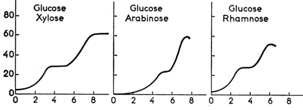
When exploring the fascinating ways in which bacteria and namelyEscherichia coli adapt to their surrounding environments, we must acknowledge that we are standing on the shoulders of giants and give nod to the foundational work that began nearly 80 years ago by Jacques Monod. From a now seemingly simple experiment of providing bacteria with two sugars (glucose and arabinose for example), Monod discovered an interesting pattern of growth, resulting in the famed diauxic growth curves (Figure 1.1). Such growth curves are distinguished by two distinct growth phases, one where the preferred sugar (glucose in this case) is metabolized, followed by growth on the secondary sugar. The transition between the two growth phases can clearly be seen as a distinct secession of growth, a period of “adaptation". The mystery presented by these growth curves is precisely what is occurring in the cells during this period of adaptation.

(12)

Figure 1.1: Examples of diauxic growth from Monod’s thesis (1941), as reproduced in Monod, 1966. The x-axis is time in hours and the y-axis is optical density (arbitrary units), a metric of cell growth.

As Monod recalls in reflecting on his initial discovery, his colleague André Lwoff at the time suggested that it might have something to do with “enzymatic adaptation”

(Monod, 1966), the idea that some protein already present in the cell responds to the changes in relative sugar concentrations. And thus the notion of adaptation on the molecular level was created. While the idea that enzymes themselves can change in response to surroundings (e.g. activity changed in response to the binding of the ligand), the primary cause of the lag in growth was due not to protein response alone, but to the need for a new suite of genes to be expressed and produced in response to the change in sugar. Monod’s original discovery led to a decades-long journey of teasing apart how such gene regulation is enacted.

Next we will discuss the broad strokes nature of gene regulation, the way in which the expression of given genes can be modulated by the binding of proteins to DNA known as transcription factors. By way of example, we will specifically consider the extensively studiedlacoperon here, but many other genes have undergone similar dissection.

A note on adaptation

As a quick aside, I want to riff on an alternate meaning of adaptation. While thus far we have discussed what could be referred to asphysiological adaptation, the perhaps more common use of the word adaptation is within the context of evolutionary adaptation. Examples of adaptations in this context would be the formation of webbed feet to aid in swimming or the use of prehensile tails for effective climbing in trees. The timescales required for these incredible feats to have evolved are nearly irrelevant for our present discussion regarding molecular

(13)

adaptation and the ways in which cells respond in real time to their surroundings.

While the concept of evolutionary adaptation is not the primary focus of this thesis, it is important to note that the molecular mechanisms that are in place to permit cells to readily adapt to their surroundings are themselves subject to natural selection. As such, the ability to adapt is itself an adaptation, but for now, we focus our efforts on how cells enact their molecular adaptation rather than how such adaptions arose in the first place.

1.3 The molecular players of gene regulation: thelacoperon as an example With decades of painstaking experiments, the field of molecular genetics was able to make sense of the diauxic curves that Monod first discovered in the 1940s. In the specific case of cells provided with glucose and lactose, the molecular mechanisms of diauxic growth are illustrated in Figure 1.2. While specifically these lactose metabolizing genes are the primary focus of this section and arguably the most well-studied gene inE. coli, the mechanisms discussed here have far broader reach than just this single set of genes in this single organism. Most notably, our primary focus will be on a suite of proteins known as transcription factors, which bind to DNA and accordingly influencing the level of transcription (i.e. gene expression).

Within the class of transcription factors, these proteins either act as activators to increase transcription orrepressorsto prevent or lower transcription. As an aside, it is possible for a given transcription factor to act as both an activator and a repressor, a duality known as a ‘Janus molecule’. However, this switch from activation to repression is mediated by some environmental cue, still making it reasonable to break transcription factors into these two discrete groups at least when considering a given gene and a given environment.

By way of example, we will work through the logic of thelac operon, illustrating the roles that activators and repressors can play in mediating the level of gene expression. Conveniently, the lacoperon has one activator and one repressor that modulate its expression, making it a useful example to work though. As a way to understand the regulatory logic of this operon, it is important to remember that the lac operon encodes a number of genes involved in lactose metabolism, thus it make sense that the cell would only ‘want’ these genes to be turned on in the presence of lactose. Indeed, we can see that this is precisely how the regulation of the lac operon is enacted, with the repressor bound when there is no lactose around (Figure 1.2). With this set up, these lactose metabolizing genes will not be needlessly produced when their target substrate is not present. Conversely, as

(14)

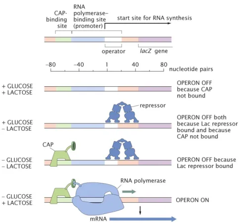
Figure 1.2: Regulation of thelacoperon. The top schematic illustrates the key DNA regions of thelacoperon. The GLUCOSE and LACTOSE labels on the left indicate the four possible environmental conditions in the presences (+) or absence (-) of these sugars, with the resulting regulatory state on the right. From this, we can see that the lacgenes are only actively transcribed in the presence of lactose and the absence of glucose. Figure reproduced fromPhysical Biology of the Cell.

hinted by the shape for the diauxic growth curves, there are some sugars that are preferred over others. Specifically, glucose is the most preferred sugar as it can be immediately consumed through the citric acid cycle, while other sugars are only metabolized as an alternative. With this stipulation in mind, the cell would also ‘want’ to not express the lactose metabolizing genes when there is a perfectly more suitable sugar around such as glucose. Examining Figure 1.2, we can see that such logic is encoded molecularly through the use of the catabolite activator protein (known as CAP). That is, only in the absence of glucose does CAP serve to promote transcription by binding upstream of the lacpromoter. Together through the action of the LacI repressor and the CAP activator, the regulation of these genes are effectively controlled as an AND gate, whereboth the presence of lactoseand the absence of glucose are required for transcription.

(15)

While I am glossing over decades worth of hard-earned results as summarized by a single figure, it suffices to say that it is in fact possible to gain such a detailed understanding of how a given gene is regulated, i.e. which transcription factors are binding, where they bind, and whether they act as an activator or repressor. The next section will delve into what we can do with such a regulatory model in hand.

1.4 Statistical mechanics of gene regulation

As will be a common theme throughout this thesis, we will argue for moving beyond a qualitative understanding of gene regulation, as typified by the ‘cartoon’

models, like those in Figure 1.2. Instead, we would would like to be able to have a mathematical model in addition to our pictorial one. The reason is simple: data in molecular biology are becoming ever more quantitatively precise, and accordingly our hypotheses should be similarly precise. For this, we will rely on an a physical framework known asstatistical mechanics. This section provides a brief overview of how the tools of statistical mechanics can be brought to bear on gene regulation.

A key tenet of statistical mechanics is described by Boltzmann distribution which states that the probability of a given state occurring is

𝑃_state = 𝑒

−^𝜖^state

𝑘 𝐵𝑇

Z , (1.1)

where𝜖_{𝑠𝑡 𝑎𝑡 𝑒} is the energy associated with the state, 𝑘_𝐵 is the Boltzmann constant, and𝑇 is the temperature, andZ is known as the partition function, or the sum of the probabilities of all possible states. In words, this equates to lower energy states being more likely to occur and higher energy states becoming vanishingly less likely to occur, due to the exponent. We can make sense of this intuitively to explain why we don’t spontaneously begin levitating. The energy, specifically the potential energy 𝑚 𝑔 ℎ, associated with the “state” of levitating is simply too large for it to realistically ever occur for large masses𝑚such as ourselves. Now we must contend with what exactly is meant by a ‘state’ in statistical mechanical sense, starting with an example of RNA polymerase (RNAP) binding to DNA.

A state is some condition that we are interested in assessing the frequency of, such as whether an RNAP is bound to a promoter of interest. An additional definition is that a microstate is simply one specific manifestation of a state of interest. As illustrated in the bottom panel of (Figure 1.3), there are many ways to realize the binding of RNAP to DNA, each one its own microstate. Specifically, if we discretize

(16)

the genome, which is not an unreasonable assumption given that RNAP binds in register with specific basepairs, there end up being a total of𝑁_{𝑁 𝑆}nonspecifc binding sites for the𝑃polymerases to find themselves. The task at hand is to enumerate all these possible microstates, which can be defined as

𝑊(𝑃, 𝑁_{𝑁 𝑆})= 𝑁_{𝑁 𝑆}

𝑃

= 𝑁_{𝑁 𝑆}!

𝑃!(𝑁_{𝑁 𝑆}−𝑃)!, (1.2) where we use the notation that𝑊 stands for the number of microstates.

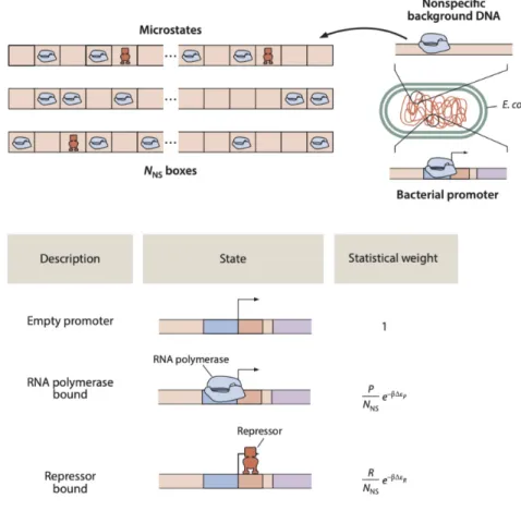
Figure 1.3: Microstates of RNA polymerase binding to DNA. The top panel schema- tizes the cell’s pool of RNA polymerase (RNAP) as bound in various location along the length of the bacterial (circular) genome. The bottom panel illustrates three specific realizations (i.e. microstates) of the ways in which the RNAP may allocate themselves within the 𝑁_{𝑁 𝑆} ‘boxes’ or basepairs of the genome. Figure reproduced fromPhysical Biology of the Cell.

With the enumeration of the states, along with Boltzmann distribution (Equa- tion 1.1), we are poised to assess the probability of a promoter being bound by RNAP. That is, the probability of a state occurring is a function of both its associated energy (as prescribed by the Boltzmann distribution)andthe number of ways in which a given state can occur, known as themultiplicity. Put together, we end up with the partial partition function for nonspecific binding as

(17)

Z𝑁 𝑆(𝑃, 𝑁_{𝑁 𝑆}) = 𝑁_{𝑁 𝑆}! 𝑃!(𝑁_{𝑁 𝑆}−𝑃)!

| {z }

multiplicity

× 𝑒⁻

𝛽 𝑃𝜖^{𝑁 𝑆}

| {z }𝑝 𝑑

Boltzmann factor

, (1.3)

where we have introduced the simplifying notation that𝛽=1/𝑘_𝐵𝑇and have defined 𝜖^{𝑁 𝑆}

𝑝 𝑑 as the binding energy of polymerase to DNA at a nonspecific location. What Equation 1.3 describes is the probabilistic weight associated with all𝑃polymerases being bound nonspecifically. However, if we are interesting in when a gene is being actively expressed, we would want to assess the probability that a polymerase is in fact bound to the promoter we are interested in, as schematized in Figure 1.4.

That is, we want to compare the probabilistic weight of the promoter being bound relative to all possible states (promoter bound or unbound). For obtaining the partial partition function for polymerase being bound to the promoter, this amounts to effectively taking one polymerase out of circulation and placing the remaining 𝑃−1 polymerases on the𝑁_{𝑁 𝑆}genome positions. This results in the following partial partition function for when a polymerase is bound to the promoter of interest:

Z𝑁 𝑆(𝑃−1, 𝑁_{𝑁 𝑆}) = 𝑁_{𝑁 𝑆}!

(𝑃−1)!(𝑁_{𝑁 𝑆}− (𝑃−1))!

| {z }

multiplicity

×𝑒^{−𝛽(𝑃−1)𝜖}

𝑁 𝑆 𝑝 𝑑𝑒^−𝛽𝜖

𝑆

| {z }𝑝 𝑑

Boltzmann factor

. (1.4)

Figure 1.4: Pictorial representation of 𝑝_bound. The numerator is the sum of all the microstates in which the promoter of interest is bound by polymerase. The denominator is the sum all all states (i.e. those where the promoter is occupied and those where the promoter is unoccupied). Figure reproduced fromPhysical Biology of the Cell.

Note how the multiplicity is described by placing𝑃−1 polymerases, and the Boltz- mann factor now also has𝑃−1 instances of nonspecific binding in addition to one

(18)

instance of specific binding, with energy 𝜖^𝑆

𝑝 𝑑. These computations of the probabilistic weights are illustrated in Figure 1.5. We can simplify the multiplicities slightly by making the approximation𝑁_{𝑁 𝑆}!/(𝑁_{𝑁 𝑆}−𝑃)!≈ (𝑁_{𝑁 𝑆})^𝑃, with the reasonable assumption that 𝑃 𝑁_{𝑁 𝑆}. This approximation leaves us with the following weights:

Z𝑁 𝑆(𝑃, 𝑁_{𝑁 𝑆})= (𝑁_{𝑁 𝑆})^𝑃 𝑃! 𝑒⁻

𝑝 𝑑, (1.5)

and

Z𝑁 𝑆(𝑃−1, 𝑁_{𝑁 𝑆}) = (𝑁_{𝑁 𝑆})^𝑃−1 (𝑃−1)! 𝑒⁻

𝛽(𝑃−1)𝜖^{𝑁 𝑆}

𝑝 𝑑𝑒⁻

𝛽𝜖^𝑆

𝑝 𝑑. (1.6)

Figure 1.5: States and weights for polymerase binding. The top panel works through the computation for the Boltzmann weight for the state of the promoter of interest being unoccupied by polymerase. By contrast, the bottom panel computes the weight for an occupied promoter. Figure reproduced fromPhysical Biology of the Cell.

At long last we are equipped to assess the probability that the promoter is in fact bound by polymerase, a state we will use as a proxy for gene expression. With Figure 1.4 as a visual aid for how to compute 𝑝_bound, we arrive at

𝑝_bound=

(𝑁_{𝑁 𝑆})^𝑃−1

(𝑃−1)! 𝑒^{−𝛽(𝑃−}¹^)𝜖

𝑁 𝑆 𝑝 𝑑𝑒^−𝛽𝜖

𝑆 𝑝 𝑑

(𝑁_{𝑁 𝑆})^𝑃 𝑃! 𝑒⁻

𝑝 𝑑 + ⁽^𝑁₍^{𝑁 𝑆}⁾^𝑃−¹

𝑃−1)! 𝑒⁻

𝛽(𝑃−1)𝜖^{𝑁 𝑆}

𝑝 𝑑 𝑒⁻

𝛽𝜖^𝑆

𝑝 𝑑

, (1.7)

which is fairly daunting at first sight, but many values cancel out, leaving us with

(19)

𝑝_bound = 1 1+ ^𝑁^{𝑁 𝑆}

𝑃 𝑒^𝛽^Δ^𝜖^{𝑝 𝑑}

, (1.8)

whereΔ𝜖_{𝑝 𝑑} is defined as the difference between specific and nonspecific binding.

Figure 1.6: States and weights for simple repression. Figure adapted from Phillips et al., 2019.

While all this effort for modeling constitutive gene expression may seem rather arduous, there is great utility in this statistical mechanical protocol outlined here.

If we wish to add the action of some transcription factor binding, say a repressor, it is actually quite simple to do so. The derivation we went through here applies by analogy to any protein binding to DNA. It is precisely the regulation enacted by a single repressor (a motif known as simple repression) that was the focus of work done by Brewster et al., 2014. While we won’t go through the whole derivation again, we can use the same approaches outlined here for the constitutive promoter to arrive at the states and weights as shown in Figure 1.6.

(20)

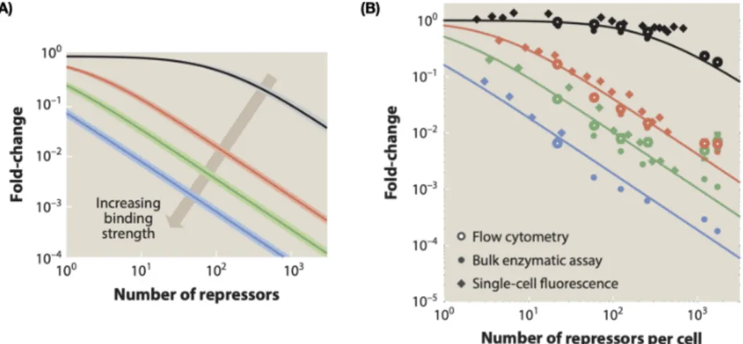
It is with these states and weights in hand, we can now formulate a concrete mathematical prediction of how gene expression should change as a result of increasing repressor counts. It is precisely this theory-experiment dialogue that was conducted to much avail by Brewster et al., 2014, as shown in Figure 1.7. Such experiments serve to give us the sense that these statistical mechanical models of gene expression do actually fare well in describing the data. These careful mathematical models require knowing the precise regulatory structure of the promoter of interest, which works well for the thoroughly studiedlacpromoter. As we will see in the following section, however, there remain many genes for which such a treatment is not yet possible.

Figure 1.7: Theory meets experiment for simple repression. (A) Shows the prediction of how gene expression should change with increasing number of repressors, for four different binding sites. (B) Shows how the various data land relative to these predictions. Figure adapted from Phillips et al., 2019.

1.5 On our regulatory ignorance

Now that we have a cursory sense of the ways in which genes have been shown to be regulated and how we might mathematically model them, we come to one of the primary motivations of the work of this thesis: despite how much effort has been put into understanding how genes are regulated, especially in E. coli, there still remain many genes for which we know nothing regarding how they are regulated. Figure 1.8 (A) concisely illustrates the extent to which we remain ignorant of regulation even in the best case scenario ofE. coli. Prior to the work conducted in this thesis, nearly two-thirds of all operons had no annotated gene regulation (i.e.

any transcription factor binding sites), as annotated on RegulonDB Santos-Zavaleta

(21)

et al., 2019. (It’s important to note that this value stated here includes the work done by Ireland et al., 2020, and that the number of genes with no known regulation was actually even greater prior to the work done in this thesis, as can be seen in Figure 2.1.) Unfortunately, as the remaining panel of Figure 1.8 reveal, the status of our regulatory ignorance only becomes worse as we move to higher organisms.

E. coli S. cerevisiae

D. melanogaster

C. elegans

4

chromosome

3 2

X 4

3 2 1

5 X

10 Mbp

16 15 14 13 12 11 10 9 8 7 6 5 4 3 2 1 chromosome

200 kbp

E. coli genome oriC

1 Mbp

2 Mbp

3 Mbp 4 Mbp

?

lac operon well characterized promoter yaiL operon

no known binding sites

5 Mbp 62%

94.8%

38%

96.4%

99.9%

genes with known regulatory DNA sequences genes with no known

regulatory DNA sequences

3.6%

5.2% 0.1%

(A) (B)

(D)

(C)

Figure 1.8: Regulatory ignorance across the domains of life. This schematized view of several genomes, showing each gene for which there is any known regulation (blue dashes) as opposed to those for which there was no known regulation (red dashes).

This schematic shows our level of regulatory ignorance across (A)E. coli, (B) the budding yest,Saccharomyces cerevisiae, (C) the fruit flyDrosophilia melanogaster, and (D) the nematodeCaenorhabditis elegans.

The primary battle cry of this thesis is that, as seen with thelacoperon, we need to know some basic facts about the regulation of a given operon before we can begin to conduct the careful quantitative dissections discussed here. Thankfully, previous work can shed light on where regulation may be occurring even if we don’t yet know

(22)

the details of that regulation. One such set of key experiments were conducted by Schmidt et al., 2016, where they assessed the fullE. coliproteome over 22 unique growth conditions. By examining proteins whose expression changes dramatically across growth conditions, we can gain insight into genes whose expression likely seems to be regulated (and thus is only turned on in one or few conditions). As Figure 1.9 illustrates, there are in fact many proteins whose expression is highly variable across these 22 growth conditions, and with respect to our mission to explore the currently unannotated genes, we are heartened to see that both genes with known (in blue)and no known (in red) regulation demonstrate variable gene expression. It is precisely these genes in red with high coefficient of variation that serve as ideal candidates for uncovering hitherto unexplored regulation. Precisely how we do achieve that goal is introduced in the following section and is the primary thrust of the remainder of this thesis.

Figure 1.9: Evidence of gene regulation in unannotated genes. Each protein (categorized as having annotated regulation in blue or no known regulation in red) are plotted according to their coefficient of variation across the 22 growth conditions tested in Schmidt et al., 2016. Plots adapted from Belliveau et al., 2018.

1.6 From dissection to exploration

With the widespread issue of regulatory ignorance laid out clearly before us, we must now contend with how we can go about uncovering such previously unexplored genes. Work pioneered by Kinney et al., 2010 served to establish the Sort-Seq method, which Belliveau et al., 2018 later used to great avail to unveil

(23)

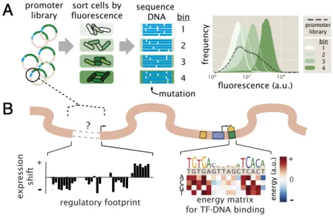
the regulation of some previously unexplored genes. The protocol is outline as in Figure 1.10. In brief, the scheme is to take a promoter region of interest and make a mutagenized library of promoter variants all driving expression of some fluores- cent protein reporter gene. Using fluorescence-activated cell sorting (FACS), the initially heterogeneous population of cells can be separated into four distinct bins (Figure 1.10 (A)). The cells in each bin are then sequenced, allowing us to build up a picture of which mutations confer changes in fluorescence.

Figure 1.10: The Sort-Seq protocol. (A) By mutagenizing a promoter region of interest driving expression of some reporter protein, we can obtain cells with varying levels of fluorescence. These cells are sorted via flow cytometry into four bins and each bin is independently sequenced. The plot on the right shows the distribution of fluorescence of the four bins after having been sorted, demonstrating that the difference in gene expression is maintained within the disparate bin population.

(B) With the sequencing information in hand, we can begin to assess the relative importance that each basepair has with respect to the level of gene expression. This formation is computed and displayed as expression shift plots (on the left) and energy matrices (on the right).

Specifically, along the length of the promoter region of interest, it is possible to assess whether a given basepair increases or decreases expression upon being mutated.

Such information leads to an expression shift profile, as shown in left of Figure 1.10 (B). Such a plot gives a gives a quick visual aid as to where transcription factors may be binding, as these regions are the most likely to have an impact on the level of expression. For example, if a given mutation disrupts the ability of a repressor to bind, we would expect such a variant to have higher gene expression than normal.

(24)

However we can also take a more detailed look at a given binding, as depicted by an energy matrix (right panel, Figure 1.10 (B)). Using the tools of statistical mechanics as outlined in Section 1.4, it is possible to directly connect the changes in gene expression to a binding energy. In this way, we are able to determine not just which basepairs are involved in regulating expression, but we can also concretely predict what effect various mutations will have.

With this technique in hand, it is essential to evaluate its ability to recover known regulation if it is to be of any use in uncovering our regulatory ignorance. By way of example, we once again return to thelacoperon, whose regulation is well understood.

Hearteningly, Belliveau et al., 2018 were in fact able to recover the known regulation for the promoter region when giving it the full Sort-Seq treatment, as revealed by the expression shift plot (Figure 1.11). Walking through these results, we can see that mutating the region where the lacI repressor binds causes the expression to go up on average. This makes sense as disrupting the binding of lacI will lead to a failure to repress the gene, ultimately causing gene expression to be higher. Conversely, we see that the regions where CAP and RNAP polymerase show the opposite effect, where mutation led to lower expression.

Figure 1.11: Expression shift for the mutagenized lac promoter. The plot show the average effect of mutating a given position with respect to the resulting gene expression. The colored bars above the plot denote where the known binding sites are located. Data and figure from Belliveau et al., 2018.

These results encourage us that we can in fact use the Sort-Seq method to unveil gene regulation. In fact, the remainder of the work done by Belliveau et al., 2018 served to dissect two other promoters with known regulation and importantly four promoters with previously no known regulation. This incredibly important study served as an essential proof of concept as we embarked on the work discussed in this thesis. From here, we sought to expand the utility of Sort-Seq from dissecting

(25)

a single promoter at a time to being able to explore ten and even one hundred promoters at a time.

1.7 A primer on mutual information

Whether we are measuring fluorescence of a reporter protein or mRNA counts, we must now contend with how to make sense of the data in hand, specifically how to relate sequence identity to gene expression. For this we turn to the concept of mutual information, a metric by which we can understand how much information one variable provides about another. In this case, we would be interested in how much information a given DNA sequence gives us with respect to the resulting level of gene expression. Concretely, the mutual information between two discrete random variables𝑋 and𝑌 is defined as

𝐼(𝑋;𝑌) =Õ

𝑦∈𝑌

Õ

𝑥∈𝑋

𝑝(𝑥 , 𝑦)log

𝑝(𝑥 , 𝑦) 𝑝(𝑥)𝑝(𝑦)

, (1.9)

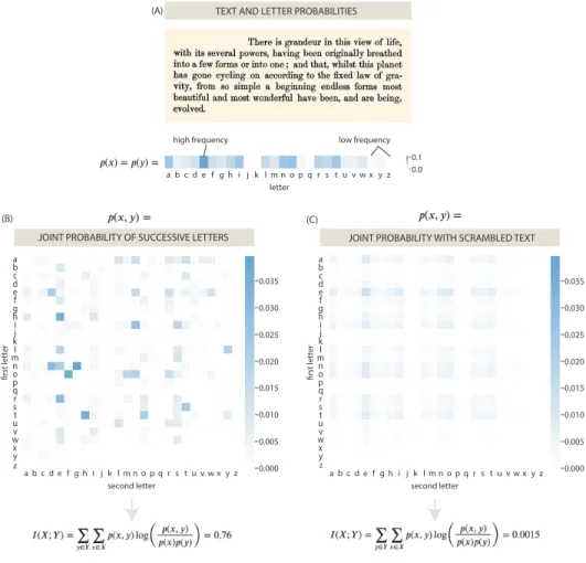
where 𝑝(𝑥 , 𝑦) is the joint probability of𝑥 and𝑦 occurring. To gain more intuition into what this actually means, let’s walk through an example that will be more familiar before delving into the case of gene expression. Let’s take an iconic piece of text from the final sentence of Darwin’sOn the Origin of Species:

"There is grandeur in this view of life, with its several powers, having been originally breathed into a few forms or into one; and that, whilst this planet has gone cycling on according to the fixed law of gravity, from so simple a beginning endless forms most beautiful and most wonderful have been, and are being, evolved."

As an exercise, we can ask what the mutual information is between subsequent letters in this piece of text. That is, how much information does one letter give us about what letter is likely to follow? As prescribed in Equation 1.9, to compute the mutual information, we need both the joint probability of the two variables, 𝑝(𝑥 , 𝑦) as well as their individual probabilities, 𝑝(𝑥) and 𝑝(𝑦), respectively. Figure 1.12 (A) illustrates these frequencies of each letter as found in this text. Intuitively, we can see that the letter ‘e’ is in fact the most common letter, and from here, we can begin to assess the joint probabilities as shown Figure 1.12 (B). Once again, we can make sense of the results shown here by noting the ‘t’ followed by ‘h’ as well ‘h’

(26)

z

0.1 a b c d e f g h i j k l m n o p q r s t u v w x y z 0.0

letter

a ab cd ef gh ij kl mn op qr st uv wx y

b c d e f g h i j k l m n o p q r s t u v w x y z second letter

first letter

high frequency low frequency

0.035 0.030 0.025 0.020 0.015 0.010 0.005 0.000

z a

ba dc ef gh ij kl mn op qr st uv wx y

b c d e f g h i j k l m n o p q r s t u v w x y z second letter

first letter

0.035 0.030 0.025 0.020 0.015 0.010 0.005 0.000 JOINT PROBABILITY OF SUCCESSIVE LETTERS JOINT PROBABILITY WITH SCRAMBLED TEXT

TEXT AND LETTER PROBABILITIES (A)

(B) (C)

Figure 1.12: An example of mutual information on a piece of text. (A) The text from the final sentence of Darwin’sOn the Origin of Species, along with the frequencies with which each letter appears. (B) The joint probabilities of two consecutive letters from the original text. (C) The joint probabilities of two consecutive letters when the text has been scrambled.

followed by ‘e’ are the most common, as expected by the common use of the word

‘the’.

Intuitively, we can see that there is in fact some information contained in this piece of text with regards to the identity of two consecutive letters. That is, if you were given a letter, you would be able to make a reasonable guess about which letter will follow (performing at least better than guessing randomly). To be more quantitatively precise, we can now plug in both the basal letter probabilities, both 𝑝(𝑥) and 𝑝(𝑦) in this case as shown Figure 1.12 (A) and the joint probabilities form Figure 1.12 (B) into Equation 1.9 to arrive at the total mutual information.

Mechanistically, this entails looping through all possible letter combinations and

(27)

assessing both their joint probability 𝑝(𝑥 , 𝑦) and their ‘expected’ probabilities of simply multiplying their independent frequencies together, 𝑝(𝑥) × 𝑝(𝑦). From this calculation, we arrive at value of 0.76 (Figure 1.12 (B)). However, to make sense of what this number means, we can by way of contrast scramble the text and repeat the procedure, as shown in Figure 1.12 (C). Such scrambled text might look something like this:

"pgfsfw ledeu e dtrxeiieui vh vtatbbetawo oo fear.di,n nor fsrmo ev ot iaernvbws o,f lfmcatgs ebeeleruiim,tse rwohardntot dbo fctby r nndatla f ndn in hhie ncei roocs nvn aaa, leml oes aselee uc.dhpdnltwan yeaai htcghus xowfhgo w, iltenrhoerwaccsrau ftg;,h nedsr mmoo pon oeoer- wioerid oit enohantosnrortgge hhhg enfttliem ylln, hwer le w,oa nmfi- belhea ,a hfdaoo,lsna uiile fgmcsatt pifaos,loavieeocareiefnefynenn etj s hair pgtfin ilteeyghiitrcl hdh imsttblvsanrt,i sg o vdaiedtmman ise"

We can intuit that this piece of text has now sadly been rendered meaningless. We can see this more precisely in Figure 1.12 (C) that there are no letter combinations that are favored and ‘e’ becomes the most likely letter to follow regardless of the previous letter, as it is simply the most common letter. Lastly, we can quantify this by again making use of Equation 1.9. We now see that the mutual information is 0.0015, nearly 0, which would imply no information, as expected when the text has been scrambled and all the original meaning as been lost.

With what I hope is a more intuitive example in mind, we can finally return to the primary scientific question at hand: how much information does knowing a given DNA sequence give us about the resulting gene expression? As illustrated with a toy example in Figure 1.13, we can use the same exact approach to assess the joint probabilities between the identity of a given DNA nucleotide (A, T, C, or G) and the resulting gene’s expression (as measured by binning according the fluorescence level). In Figure 1.13, the first position can be seen to contain a high information, as knowing the identity of the nucleotide permits you to make a suitable guess as to which level of expression the DNA will promote. However, position 2 would have low information, as the joint probabilities are much more uniform and no single bin is particularly favored over another. By repeating this calculation over every nucleotide position along the length of DNA region of interest, we can begin to build a picture of which bases are most important for determining the level of expression.

Such bases that are found to contain more information are thus heavily implicated

(28)

Figure 1.13: An example of mutual information between DNA sequence and gene expression. Tables show the joint probabilities between nucleotide identity along thes rows and gene expression along the columns. The level of gene expression is discretized into bins, with increasing fluorescence indicated with intensity in green. Intensity in purple represents the value of the joint probabilities. Position 1 demonstrates high mutual information between the identity of the nucleotide and the level of gene expression (i.e. bin). By way of contrast, position 2 demonstrates lower mutual information as the joint probabilities are much more uniform.

in serving some regulatory role, such as serving as a binding site for a transcription factor. In the chapter that follows, it is precisely this approach that will be brought to bear on deciphering the yet-to-be understood regulatory regions of the E. coli genome.

1.8 In conclusion: where we go from here

With this introduction I hope I have impressed upon you two key themes: 1) the universality of adaptation, and specifically gene regulation as a lens through which to understand how cells adapt to their surroundings and 2) the need for a quantitative understanding of how gene regulation is enacted. However, as a first pass we need to know which transcription factors are even involved as well as where and how strongly they bind to a given promoter. With these motivating points in mind and a few “tricks of the trade” (i.e. statistical mechanics and mutual information) in hand, we are prepared to tackle the problem of our regulatory ignorance inE. coli. What follows is the magnum opus of my thesis, where we brought these tools to bear in deciphering a substantial chunk of theE. coligenome, one hundred genes in one set of experiments.

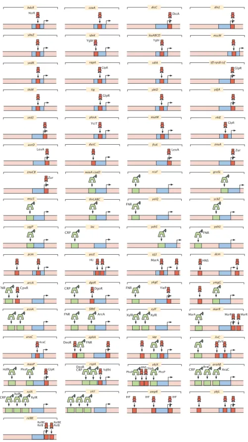
The results of my thesis can be concisely summarized in Figure 1.14. While the precise details of how these cartoon models were elucidated is left to Chapter 2,

(29)

bdcR NsrR

coaA dicC

DicA

dinJ

ybeZ idnK

YgbI

leuABCD YgbI

mscM

yedK rapA

GlpR

sdiA tff-rpsB-tsf

GlpR

thiM tig ybiO

GlpR

ydjA

yedJ

YciT

phnA mutM rhlE

GlpR

LexA

uvrD dusC

LexA ftsK

Zur znuA

znuCB Zur

waaA-coaD rcsF groSL

mscS thrLABC yeiQ

FNR

ycbZ

ygjP

CRP

lac yehS

FNR yehU

pcm yecE

HU

yjjJ MarA

dcm HNS

arcA

FNR CpxR CRP DgoR

dgoR

YieP FNR

ykgE ymgG

asnA

FNR ArcA

fdhE xylF

XylR XylR ^MarA ^MarR ^MarR

marR

AraC araC

DeoR FNR

aphA iap

IlvY ilvC

maoP GlpR PhoP

HdfR DeoR

CRP YdfH

rspA ybjX

PhoP HNS StpA PhoP

araAB AraC AraC CRP

xylA XylR

CRP XylR ^yicI

IHF IHF

ompR IHF

ybjL

RelBE RelB RelBERelB relBE

Figure 1.14: All regulatory architectures uncovered in this study. (Continued on the following page.)

(30)

Figure 1.14: For each regulated promoter, activators and their binding sites are labeled in green, repressors and their binding sires are labeled in red, and RNAP binding sites are labeled in blue. All cartoons are displayed with the transcription direction to the right. Only one RNAP site is depicted per promoter. Binding sites found for these promoters in the EcoCyc or RegulonDB databases are only depicted in these cartoons if the sites are within the 160 bp mutagenized region studied, and were detected by Reg-Seq.

this figure shows every binding site that was discovered across the 113 promoters explored here. It important to note that the cartoon models shown here belie the precise quantitative backing that supports these results. That is, each binding site has its own information footprint and energy matrix as with the traditional Sort-Seq approach outlined in Figure 1.10. This means that not only do we know where transcription factors are binding, how they are regulating (i.e. as an activator or repressor), and in many cases the identity of the transcription factor, but we also know how strongly the given transcription factor binds. It is with this deep quantitative understanding of how these genes are regulated that we can make predictions as seen in Figure 1.7 and begin to test our understanding of how regulation is enacted well beyond what is illustrated by a cartoon alone.

The work discussed here has transformed the utility of Sort-Seq from being able to elucidate single genes to over a hundred genes at a time. With around 4000 genes in theE. coli, we can see a path to having the entire regulatory genome ‘solved’ within the coming years, hopefully radically transforming the view of Figure 1.8 (A). For now though, let’s dive into this first feat of tackling one hundred promoters.

(31)

C h a p t e r 2

DECIPHERING THE REGULATORY GENOME OF ESCHERICHIA COLI, ONE HUNDRED PROMOTERS AT A

TIME

Published as:

Ireland, W. T., S. M. Beeler, E. Flores-Bautista, N. S. McCarty, T. Röschinger, N. M. Belliveau, M. J. Sweredoski, A. Moradian, J. B. Kinney, and R. Phillips (2020). “Deciphering the regulatory genome of Escherichia coli, one hundred promoters at a time”. In:eLife. issn: 2050084X. doi:10.7554/ELIFE.55308.

arXiv:2001.07396.

2.1 Abstract

Advances in DNA sequencing have revolutionized our ability to read genomes.

However, even in the most well-studied of organisms, the bacterium Escherichia coli, for ≈ 65% of promoters we remain ignorant of their regulation. Until we crack this regulatory Rosetta Stone, efforts to read and write genomes will remain haphazard. We introduce a new method, Reg-Seq, that links massively-parallel reporter assays with mass spectrometry to produce a base pair resolution dissection of more than 100E. colipromoters in 12 growth conditions. We demonstrate that the method recapitulates known regulatory information. Then, we examine regulatory architectures for more than 80 promoters which previously had no known regulatory information. In many cases, we also identify which transcription factors mediate their regulation. This method clears a path for highly multiplexed investigations of the regulatory genome of model organisms, with the potential of moving to an array of microbes of ecological and medical relevance.

2.2 Introduction

DNA sequencing is as important to biology as the telescope is to astronomy. We are now living in the age of genomics, where DNA sequencing has become cheap and routine. However, despite these incredible advances, how all of this genomic information is regulated and deployed remains largely enigmatic. Organisms must respond to their environments through the regulation of genes. Genomic methods often provide a "parts list" but leave us uncertain about how those parts are used

(32)

creatively and constructively in space and time. Yet, we know that promoters apply all-important dynamic logical operations that control when and where genetic information is accessed. In this paper, we demonstrate how we can infer the logical and regulatory interactions that control bacterial decision making by tapping into the power of DNA sequencing as a biophysical tool. The method introduced here provides a framework for solving the problem of deciphering the regulatory genome by connecting perturbation and response, mapping information flow from individual nucleotides in a promoter sequence to downstream gene expression, determining how much information each promoter base pair carries about the level of gene expression.

The advent of RNA-Seq (Lister et al., 2008; Nagalakshmi et al., 2008; Mortazavi et al., 2008) launched a new era in which sequencing could be used as an experimental read-out of the biophysically interesting counts of mRNA, rather than simply as a tool for collecting ever more complete organismal genomes. The slew of ‘X’-Seq technologies that are available continues to expand at a dizzying pace, each serving their own creative and insightful role: RNA-Seq, ChIP-Seq, Tn-Seq, SELEX, 5C, etc. (Stuart and Satĳa, 2019). In contrast to whole genome screening sequencing approaches, such as Tn-Seq (Goodall et al., 2018) and ChIP-Seq (Gao et al., 2018), which give a coarse-grained view of gene essentiality and regulation respectively, another class of experiments known as massively-parallel reporter assays (MPRA) have been used to study gene expression in a variety of contexts (Patwardhan et al., 2009; Kinney et al., 2010; Sharon et al., 2012; Patwardhan et al., 2012; Melnikov et al., 2012; Kwasnieski et al., 2012; Fulco et al., 2019; Kinney and McCandlish, 2019). One elegant study relevant to the bacterial case of interest here by Kosuri et al., 2013 screened more than 10⁴combinations of promoter and ribosome binding sites (RBS) to assess their impact on gene expression levels. Even more recently, the same research group has utilized MPRAs in sophisticated ways to search for regulated genes across the genome (Urtecho et al., 2019; Urtecho et al., 2020), in a way we see as being complementary to our own. While their approach yields a coarse-grained view of where regulation may be occurring, our approach yields a base-pair-by-base-pair view of how exactly that regulation is being enacted.

One of the most exciting X-Seq tools based on MPRAs with broad biophysical reach is the Sort-Seq approach developed by Kinney et al., 2010. Sort-Seq uses fluorescence activated cell sorting (FACS) based on changes in the fluorescence due to mutated promoters combined with sequencing to identify the specific locations of

(33)

transcription factor binding in the genome. Importantly, it also provides a readout of how promoter sequences control the level of gene expression with single basepair resolution. The results of such a massively-parallel reporter assay make it possible to build a biophysical model of gene regulation to uncover how previously uncharacterized promoters are regulated. In particular, high-resolution studies like those described here yield quantitative predictions about promoter organization and protein-DNA interactions (Kinney et al., 2010). This allows us to employ the tools of statistical physics to describe the input-output properties of each of these promoters which can be explored much further with in-depth experimental dissection like those done by Razo-Mejia et al., 2018 and Chure et al., 2019 and summarized in Phillips et al., 2019. In this sense, the Sort-Seq approach can provide a quantitative framework to not only discover and quantitatively dissect regulatory interactions at the promoter level, but also provides an interpretable scheme to design genetic circuits with a desired expression output (Barnes et al., 2019).

Earlier work from Belliveau et al., 2018 illustrated how Sort-Seq, used in conjunc- tion with mass spectrometry, can be used to identify which transcription factors bind to a given binding site, thus enabling the mechanistic dissection of promoters which previously had no regulatory annotation. However, a crucial drawback of the approach of Belliveau et al., 2018 is that while it is high-throughput at the level of a single gene and the number of promoter variants it accesses, it was unable to readily tackle multiple genes at once. Even in one of biology’s best understood organisms, the bacteriumEscherichia coli, for more than 65% of its genes, we remain completely ignorant of how those genes are regulated (Santos-Zavaleta et al., 2019;

Belliveau et al., 2018). If we hope to some day have a complete base pair resolution mapping of how genetic sequences relate to biological function, we must first be able to do so for the promoters of this "simple" organism.

What has been missing in uncovering the regulatory genome in organisms of all kinds is a large scale method for inferring genomic logic and regulation. Here, we replace the low-throughput, fluorescence-based Sort-Seq approach with a scalable, RNA-Seq based approach that makes it possible to attack many promoters at once.

Accordingly, we refer to the entirety of our approach (MPRA, information footprints and energy matrices, and transcription factor identification) as Reg-Seq, which we employ here on over one hundred promoters. The concept of MPRA methods is to perturb promoter regions by mutating their sequences, and then to use next- generation sequencing (NGS) methods to read out how those mutations impact the

(34)

expression level of each promoter. (Patwardhan et al., 2009; Kinney et al., 2010;

Sharon et al., 2012; Patwardhan et al., 2012; Melnikov et al., 2012; Kwasnieski et al., 2012; Fulco et al., 2019; Kinney and McCandlish, 2019). We generate a broad diversity of promoter sequences for each promoter of interest and use mutual information as a metric to measure the information flow from that distribution of sequences to gene expression. Thus, Reg-Seq is able to collect causal information about candidate regulatory sequences that is then complemented by techniques such as mass spectrometry, which allows us to find which transcription factors mediate the action of those newly discovered candidate regulatory sequences. Hence, Reg- Seq solves the causal problem of linking DNA sequence to regulatory logic and information flow.

To demonstrate our ability to perform Reg-Seq at scale, we report here our results for 113E. coligenes, whose regulatory architectures (i.e. gene-by-gene distributions of transcription factor binding sites and identities of the transcription factors that bind those sites) were determined in parallel for multiple different growth conditions.

Though we make substantial progress in mapping the regulatory information for a swath ofE. coligenes in this study (the "regulome"), the field still remains limited in its understanding of which specific growth conditions, small molecules and metabolites (the allosterome) are responsible for altering the milieu of transcription factor activities (Lindsley and Rutter, 2006; Piazza et al., 2018; Huang et al., 2018).

We hope to address this shortcoming in future studies by appealing to recent work on solving the "allosterome problem" (Piazza et al., 2018). By taking the Sort-Seq approach from a gene-by-gene method to a larger scale, more multiplexed approach, we can begin to piece together not just how individual promoters are regulated, but also the nature of gene-gene interactions by revealing how certain transcription factors serve to regulate multiple genes at once. This approach has the benefits of a high-throughput assay without sacrificing any of the resolution afforded by the previous gene-by-gene approach, allowing us to uncover the gene regulation of over 100 operons, with base-pair resolution, in one set of experiments.

The organization of the remainder of the paper is as follows. In the Results section, we benchmark Reg-Seq against our own earlier Sort-Seq experiments to show that the use of RNA-Seq as a readout of the expression of mutated promoters is equally reliable as the fluorescence-based approach. Additionally, we provide a global view of the discoveries that were made in our exploration of more than 100 promoters in E.

coliusing Reg-Seq. These results are described in summary form in the paper itself,

(35)

with a full online version of the results (www.rpgroup.caltech.edu/RegSeq/

interactive) showing how different growth conditions elicit different regulatory responses. This section also follows the overarching view of our results by examining several biological stories that emerge from our data and serve as case studies in what has been revealed in our efforts to uncover the regulatory genome. The Discussion section summarizes the method and the current round of discoveries it has afforded with an eye to future applications to further elucidate theE. coligenome and open up the quantitative dissection of other non-model organisms. Lastly, in the Methods section and Appendices, we describe our methodology and the false positive and false negative rates of the method.

2.3 Results

Selection of genes and methodology

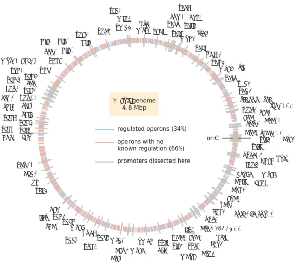
As shown in Figure 2.1, we have explored more than 100 genes from across theE.

coli genome. Our choices were based on a number of factors (see Appendix 2.6 Section “Choosing target genes” for more details); namely, we wanted a subset of genes that served as a "gold standard" for which the hard work of generations of molecular biologists have yielded deep insights into their regulation. Our set of gold standard genes islacZYA,znuCB,znuA,ompR,araC,marR,relBE,dgoR,dicC,ftsK, xylA,xylF,rspA,dicA, andaraAB. By using Reg-Seq on these genes, we were able to demonstrate that this method recovers not only what was already known about binding sites of transcription factors for well-characterized promoters (Appendix 2.7, Figure 2.14), but also whether there are any important differences between the results of the methods presented here and the previous generation of experiments based on fluorescence and cell-sorting as a readout of gene expression (Kinney et al., 2010; Belliveau et al., 2018). These promoters of known regulatory architecture are complemented by an array of previously uncharacterized genes that we selected in part using data from a recent proteomic study, in which mass spectrometry was used to measure the copy number of different proteins in 22 distinct growth conditions (Schmidt et al., 2016). We selected genes that exhibited a wide variation in their copy number over the different growth conditions considered, reasoning that differential expression across growth conditions implies that those genes are under regulatory control.

As noted in the introduction, the original formulation of Reg-Seq, termed Sort-Seq, was based on the use of fluorescence activated cell sorting, one gene at a time, as a way to uncover putative binding sites for previously uncharacterized promoters

(36)

E. coli genome 4.6 Mbp

oriC regulated operons (34%)

operons with no known regulation (66%) promoters dissected here dicB dicA

yncD hicB

ynaI ycgB

minC ymgG htrB

msyB

ybjT poxB ybiP ybiO ftsK

ybeZdpiBA ybdG tig

yajLykgE

dnaE rcsF crarapA araAB