Introduction
Dynamical tides in Jupiter as revealed by Juno
Abstract
Our results show that the gravitational effect of the dynamical tide induced by Io leads to Δ𝑘 consistent with the non-hydrostatic component reported by Juno. As a result, our results show that Juno has obtained the first unequivocal detection of the gravitational effect of dynamical tides on a gas giant planet.
Introduction
The hydrostatic tides are well constrained (i.e., the 𝑘2 error in Wahl et al. 2020 is ±0.02% of the central value) because Juno knows very precisely the effect of planet flattening on the zonal gravity coefficients 𝐽2ℓ. In Section 2, we describe the non-hydrostatic sensing of Juno and develop the mathematical formalism used in the calculation of the partial dynamical correction to 𝑘2.
Jupiter’s Love number
The tidal response of the planet causes adiabatic perturbations of the gravitational potential𝜙′, density profile𝜌′ and pressure𝑝′. The gravitational force potential 𝜙𝑇 and the tidal gravitational potential 𝜙′ are combined in ˜𝜙′ = 𝜙𝑇 +𝜙′ for analytical simplicity.
Dynamical tides in a gas giant planet
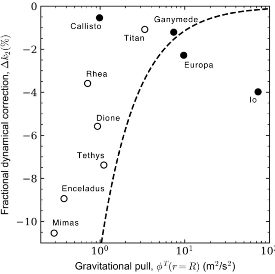
First, we solve the well-known problem of hydrostatics 𝑘2 (ie 𝜓 =0) in a sphere of uniform density (Love, 1909). 4 A partial dynamical correction applies to the 𝑛=1 polytropy caused by the gravitational force of the Galilean satellites (Eu = Europa, Ga = Ganymede, Ca = Callisto).
Discussion
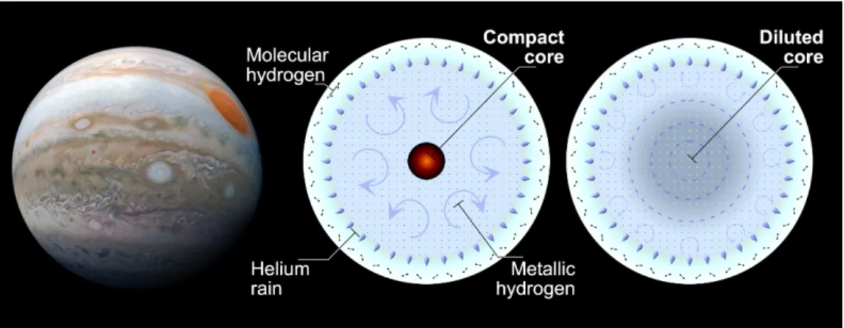
A traditional core blocks the tidal flow from extending to the center of the planet by forcing a zero flux boundary condition at the core radius. Consequently, the diluted core produces a signature in the planet's tidal response that is not recorded by 𝐽2.
Conclusions
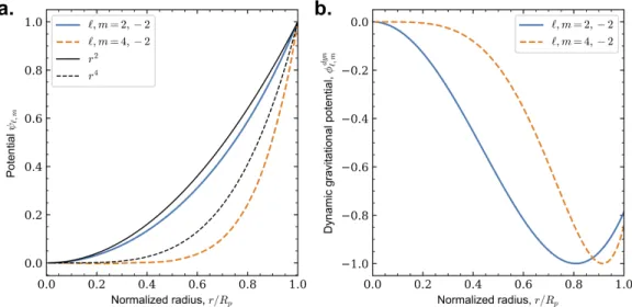
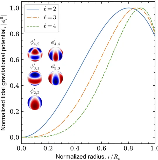
Rotation introduces a significant term with ℓ = 4 spherical harmonics corresponding to part of the tidal response to the ℓ = 2 tidal force. The oblate shape of a rotating planet introduces significant changes in the structure of the tidal gravity field.
The lost meaning of Jupiter’s high–degree Love numbers
Abstract
NASA's Juno mission recently reported Jupiter's high degree (degreeℓ, azimuthal order 𝑚 = 4.2) Love number 𝑘 𝜎), an order of magnitude above the hydrostatic 𝑘42 obtained in a non-rotating Jupiter model. After numerically modeling the rotation, the hydrostatic 𝑘 is still 7𝜎 away from the observation, casting doubt on our understanding of Jupiter's tidal response.
Introduction
As numerically shown by Wahl et al. 2020), the resulting hydrostatic Love number 𝑘42 varies greatly among the Galilean satellites with respect to the semimajor axes of each orbit, a result that contradicts the traditional concept of the hydrostatic Love number defined as a planet property. Here, we use first-order perturbation theory to analytically explain the rotation-introduced correction of the hydrostatic Love number, a result so far known only by implementing numerical strategies (Wahl et al., 2017a).
The hydrostatic tidal response
The boundary condition for𝜙′at the outer boundary of the planet defines the coefficients 𝐴ℓ. Both potentials should also match in their directional derivative normal to the outer boundary of the planet.
The hydrostatic tidal response in a rotating planet
We substitute equations (3.17) and (3.18) into equation (3.16) to obtain the final equation for the coupled hydrostatic tidal response of a planar rotating planet. 3.22) We use a recursive relation based on the Clebsch-Gordan coefficients to calculate the coupling in the spherical harmonics represented by the term𝑌𝑚. Using the recursive relation above, we can write the term that couples the spherical harmonics of the hydrostatic tidal response as .
Jupiter’s hydrostatic Love numbers
We can apply our rotational corrections calculated from equation (3.28) to the non-rotating Love numbers of a Jupiter model with a more realistic equation of state and density profile (i.e., Wahl et al. As we show here, the number the exact Love in a planet rotation comes from the boundary condition that forces the smoothness of the gravitational tidal potential on a flat planetary figure.
Discussion
Due to rotational coupling (equation (3.32)), part of the necessary correction comes from dynamical effects on 𝑘2 that include the Coriolis effect. We require future studies to understand the origin of the Δ𝑘42 fractional correction required to fit Juno observations.
Conclusions
The duration of the intra-orbital resonance and the initial dilute core structure are also uncertain. In Equation (F.2), the frequency 𝜔0 represents the 𝑓–mode oscillation frequency of the planet, which is forced by a periodic loading with frequency𝜔 associated with the gravitational pull of the companion satellite.
The gravitational imprint of an interior–orbital resonance in
Abstract
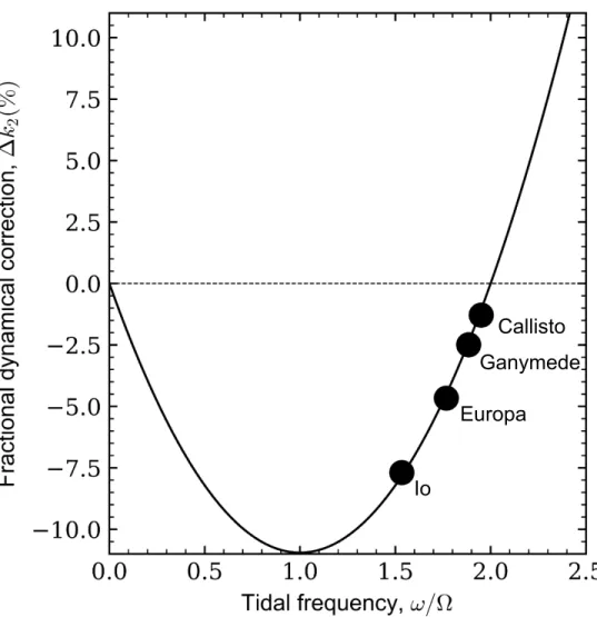
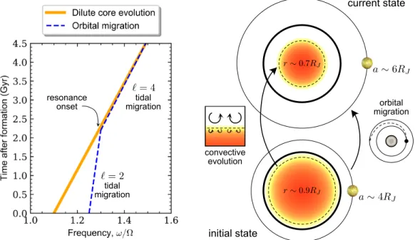
Here we propose an explanation for this puzzling disagreement based on an internal orbital resonance between internal gravitational waves trapped in Jupiter's dilute core and the orbital motion of Io. Our results show that the extended dilute core (𝑟 ≳ 0.7𝑅𝐽) causes an inner orbital resonance with Io that changes Jupiter's tidal response to Δ𝑘42 ∼ −11%, allowing us to fit Juno's 𝑘42.
Introduction
Our results support an earlier suggestion that Jupiter's dilute core may extend up to ∼0.7𝑅𝐽 (Militzer et al., 2022), without allowing us to rule out a less extended dilute core. Alternatively, a giant head-on impact could perturb Jupiter after formation, leading to an enhanced compositional gradient resistant to convective mixing (Liu et al., 2019).
An interior–orbital resonance solves the Juno discrepancy
Resonant locking is an equilibrium state where the evolution of the dilute core roughly matches the orbital migration of the forced satellite (Fuller et al., 2016). In Section 4.5 we show that the inner orbital resonance in Jupiter–Io is favored by an extended dilute core.
Jupiter dilute core models
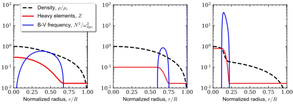
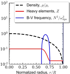
A wide diluted core with a smooth compositional gradient similar to that proposed in Debras and Chabrier (2019), (b) a narrow diluted core with a sharp compositional gradient similar to that proposed in Militzer et al. 2022), and (c) a compact dilute core with a sharp compositional gradient confined to a central region, similar to a traditional core. A compositional gradient in heavy elements introduces static stability to the interior of Jupiter, represented by the Brunt-Vaisala frequency (Fig. 4.2).
Tidal excitation of the dilute core
Our results indicate that an extended dilute core (i.e. extending as far as ≳ 0.7𝑅𝐽) produces a 24𝑔1mode frequency that resonates with the tidal frequency of the Galilean satellites (Fig. 4.4). Our compact dilute core models produce a 24𝑔1mode frequency significantly above the tidal frequency of the Galilean satellites 𝜔 < 2Ω, thus far from resonance.
Constraints to tidal dissipation imposed by resonant locking
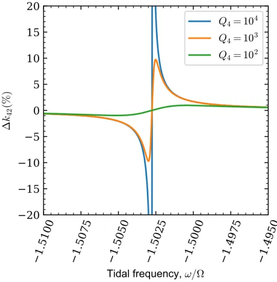
We explicitly indicate different delay angles𝛼ℓbecause dissipation can vary depending on the proximity between the tidal frequency and the mode frequency. In Equation (4.13), the relevant mode frequency is the ℓ = 2 𝑓−mode, which is much higher than the tidal frequency of the Galilean satellites and therefore leads to a relatively small𝛼4.
Discussion
Jupiter's thin core may develop as convective currents erode the thin core from above. An intra-orbital resonance with a high order24𝑔𝑛mode in a less extended dilute core (𝑟 ≲ 0.7𝑅𝐽) could alternatively explain Juno's 𝑘42 and also be maintained over geological time scales.
Conclusions
Note that equation (A.2) is non-dimensional and must be scaled by the factor. A.5) The order 𝑚 does not appear in equation (A.2), indicating a degeneracy in 𝑚 of the hydrostatic wave. We calculate the tidal flow from the design equation (2.9) in Cartesian coordinates, v=−. D.1) The potential depends on the gravitational attraction potential (2.19) and the internal tidal potential of the thin shell disturbed by tides.
Fault-zone damage promotes pulse-like rupture and back-propagating
Abstract
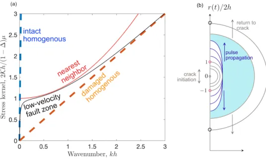
Here we show that pulses can appear in a highly damaged fault zone even in the absence of reflected waves. Furthermore, we find that slow-slip simulations in a highly flexible fault zone also propagate rearward-propagating fronts, suggesting a novel mechanism for the rapid tremor reversals observed in Cascadia and Japan.
Introduction
While the inherent complexity of large earthquakes is abundantly highlighted by modern seismological observations (Meng et al., 2012; Ross et al., 2019), reports of secondary rupture fronts propagating in the direction opposite to the main front (i.e., towards the hypocenter) are increasingly clear and robust (Beroza and Spudich, 1988; Hicks et al., 2020; Meng et al., 2011; Uchide et al., 2013; Vallée et al., 2020). Backpropagating fronts have also been identified during slow slip events (SSE) in Cascadia and Japan, which appear as tremor swarms known as Rapid Tremor Reversals (RTR) that migrate at rapid speed in the direction opposite to the propagation of the large-scale slow slip (Houston et al ., 2011).
Scaling arguments for quasi-static pulse generation
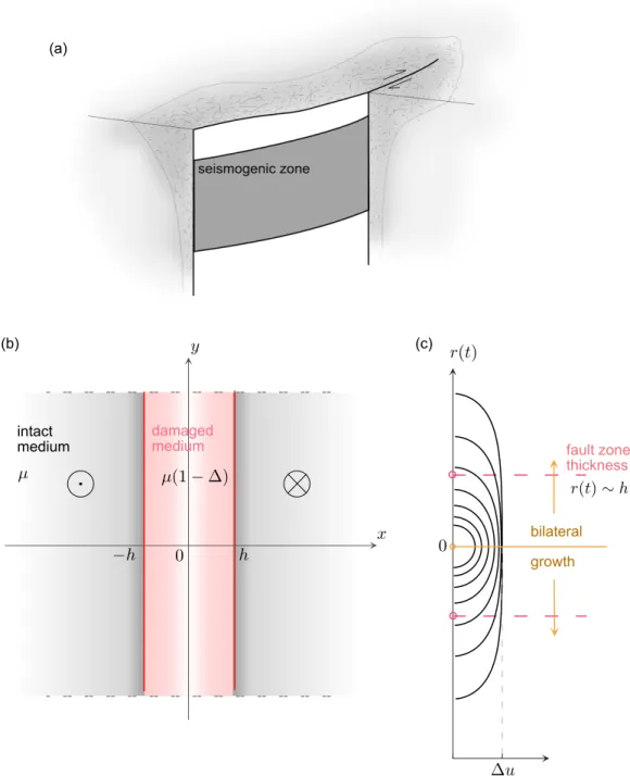
Assuming a constant fracture velocity𝑣𝑟, the size of the fracture𝑟(𝑡) is ∼𝑣𝑟𝑡, which approximately follows the rise time at the hypocenter. This rise time estimate is valid at other locations outside the hypocenter, assuming that the healing front propagation velocity is close to the fracture velocity.
Pulses and back-propagating fronts in quasi-dynamic multi-cycle
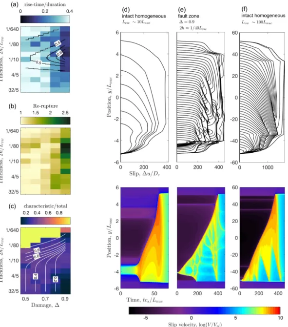
We observe a systematic reduction in the mean rise time over a wide range of LVFZ thicknesses and high damage values (Fig. 5.3a). The rupture velocity in our homogeneous medium model (Fig. 5.3d) corresponds to 𝑉𝑟 𝑢 𝑝 ∼1 km/s, a typical value in seismological observations.
Discussion
In another tectonic setting, a back-propagating front appears during a recently reported M8 intermediate-depth earthquake (Vallée et al., 2020). Preliminary results suggest that dynamic effects modulate but do not obliterate the quasi-static effects reported here (Flores-Cuba et al., 2020).
Conclusions
In relation to the left side of equation (2.14), the projections of the first, second and third terms follow respectively. B.7) The multiplication of spherical harmonics by trigonometric functions expresses a physical statement about the coupling effect that Coriolis produces in the tidal gravitational response of a rotating body. In Jupiter and Saturn, rapid rotation introduces the Coriolis effect as an important new term in the equation of motion (ie the term 2𝛀 ×v in equation F.1).
Summary of conclusions
Future research opportunities in giant planet’s interiors
A shallow fault zone structure illuminated by trapped waves in the Karadere-Duzce branch of the North Anatolian fault, western Turkey. Quantitative analysis of seismic fault zone waves in the rupture zone of the 1992 Landers, California, earthquake: evidence for a shallow trapping structure.
The Coriolis-free 𝑛 = 1 polytrope
Here we project in spherical harmonics the equation for the potential 𝜓 in a non-rotating (2.23) and rotating (2.14) 𝑛 = 1 polytrope. The equation for the gravitational potential for dynamical tides is equation (2.15), forced by a different potential depending on rotation.
The 𝑛 = 1 polytrope
Analogous to what we did for the external potential, we obtain the tidal gravitational potential (i.e.𝑟 < 𝑅𝑝) from integration throughout the volume. D.3) The constant 𝐴 comes from the numerical factor of the relevant potential, which corresponds to. Taking the continuum limit (𝑑𝑦 →0) in Eq. K.3) The second term in the right-hand side in the equation above is derived by expanding terms in a Taylor series to second order at small𝑑𝑦,.
Earthquake cycle simulations
Methods
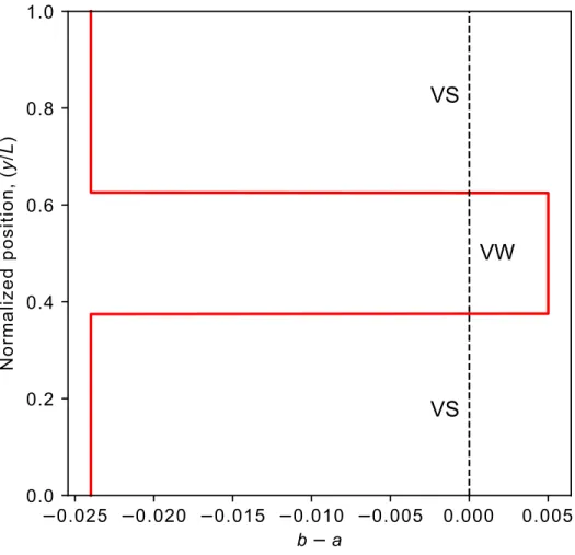
The modeling approach captures the static LVFZ effects described in Section 2 of the main text, without including any dynamic effect of fault zone reflected waves, and its computational efficiency enables a comprehensive exploration of the parameter space. The parameter 𝑎 quantifies the direct effect, 𝑏 the evolution effect, and 𝐷𝑐 is the characteristic slip related to the state evolution.
Estimation of the process zone size in a LVFZ
Problem statement
Homogeneous medium
Two-layer medium
Static slip profiles with constant stress drop
Numerical implementation of a LVFZ
Burridge-Knopoff (BK) model
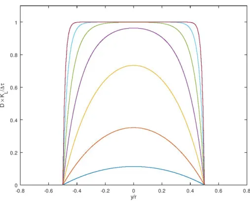
Static slip induced by uniform stress drop in the continuum BK model 118
For large values of 𝜅𝑟, the slip is flat over most of the rupture, as in pulse-like ruptures, with slip approximately equal to Δ𝜏/K¯𝐿. This shows that, under certain conditions for ℎ|𝑘|, the stress transfer of the LVFZ model is equivalent to that of the BK model, with the following formal analogies.