After the development of the integrated circuit in the 1960s, the communication channels and final speech signal processing systems changed from analog to purely digital systems. In this book, you will gain a thorough understanding of the basic scientific principles of speech production and hearing and the basic mathematical tools necessary for speech signal representation, analysis, and manipulation.
Discrete-Time Speech Signal Processing
Discrete-time signal processing is then applied to obtain the required speech modification, which is performed based on a model of speech production and a model of how articulation velocity change occurs. Timescale modification is one of the many applications of discrete-time speech signal processing that we explore throughout the text.
The Speech Communication Pathway
The pressure change at the lip, sound propagation, and the resulting pressure change at the listener's eardrum are considered the acoustic level in the speech communication pathway. Finally, at the linguistic level of the listener, the brain performs speech recognition and comprehension.
Analysis/Synthesis Based on Speech Production and Perception
In the transmitter, feedback takes place via the ear, so that one's own speech can be followed and corrected (the importance of this feedback has been shown by research into the speech of the deaf). Examples of using this feedback include controlling articulation speed and adjusting speech production to mimic voices.
Applications
Modification: The aim of speech modification is to change the speech signal in such a way that it acquires a certain desired property. Enhancement —In the third application, Speech Enhancement, the goal is to improve the quality of degraded speech.
Outline of Book
Time-frequency resolution properties of the STFT are studied and application to time scale modification is made. The wavelet transform represents one approach to address time-frequency resolution limitations of the STFT as revealed by the uncertainty principle.
Summary
BIBLIOGRAPHY
Introduction
In this chapter we review the fundamentals of discrete-time signal processing that serve as a framework for the discrete-time speech processing approaches in the rest of the text. We do not cover all relevant background material in detail, as we assume the reader's familiarity with the basics of discrete-time signal processing and given that certain topics are appropriately cited, reviewed, or expanded throughout the text as needed.
Discrete-Time Signals
Some special sequences serve as building blocks of a general class of discrete-time signals [7]. Complex exponential and top four real sequences serve as building blocks of discrete-time speech signals throughout the text.
Discrete-Time Systems
Discrete-Time Fourier Transform
Existence means that (1) X(ω) does not diverge, i.e. the Fourier transform sum converges, and (2)x[n] can be obtained from X(ω). More generally, it can be shown that the Fourier transform of a displaced ryx[n−no] is given by X(ω)e−j ωno.
Uncertainty Principle
The principle implies that a wide signal gives a narrow Fourier transform, and a narrow signal gives a wide Fourier transform.5 The uncertainty principle will play an important role in spectrographic and, more generally, time-frequency analysis of speech, particularly when the speech waveform consists of dynamically changing events or closely spaced time or frequency components. 2.7) Equation (2.7), the inverse Fourier transform of S(ω), is called the analytic signal representation of x[n] and is occasionally used later in the text.
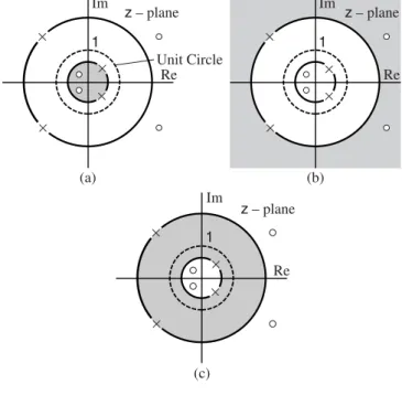
Forr = 1, the z transform becomes the Fourier transform and thus the Fourier transform exists if the ROC encompasses the unit circle. Poles are indicated by small crosses and zeros by small circles, and the ROC is indicated by shaded areas.
![Figure 2.4 Region of convergence (ROC) of the z -transform for Examples 2.5–2.7: (a) x [ n ] = δ [ n ] − aδ [ n − 1]; (b) x [ n ] = a n u [ n ]; (c) x [ n ] = − b n u [ − n − 1]; (d) x [ n ] = a n u [ n ] − b n u [ − n − 1]](https://thumb-ap.123doks.com/thumbv2/123dok/10682961.0/46.700.124.633.91.551/figure-region-convergence-roc-transform-examples-δ-aδ.webp)
LTI Systems in the Frequency Domain
Since the system is linear, we can generalize this result to the sum of sines, i.e. to enter the form. EXAMPLE 2.10 Consider again the sequence x[n] from Example 2.9 and assume that the sequence is multiplied by a Hamming window of the form [7].
Properties of LTI Systems
- Difference Equation Realization
- Magnitude-Phase Relationships
- FIR Filters
- IIR Filters
Likewise, the Fourier transform phase of a sequence of minimum phaseH(ω) uniquely specifies the sequence (within a scale factor). As we will see later in the text, there are perceptual differences in speech synthesis between the rapid and gradual "onset" of minimal and mixed phase sequences.

Time-Varying Systems
Equivalently, we can write the time-varying frequency response in terms of Green's function as (Exercise 2.17). H (n, ω)X(ω)ej ωndω (2.31) so that the output[n] ofh[n, m] at time initiates the inverse Fourier transform of the product ofX(ω) andH (n, ω), X( ω)H (n, ω) which can be thought of as a generalization of the Convolution Theorem for time-invariant linear systems.
Discrete Fourier Transform
Similar considerations must be made in frequency for the DFT realization of the Window Theorem. A more extensive description of the DFT realization of convolution theorems and windows can be found in [7].
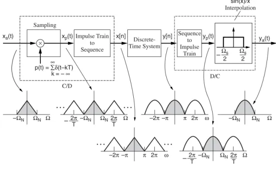
Conversion of Continuous Signals and Systems to Discrete Time
- Sampling Theorem
- Sampling a System Response
- Numerical Simulation of Differential Equations
One approach to this transformation is to simply sample the analog system's continuous impulse response; i.e. we perform the mapping continuously at discrete times. Similar to sampling continuous-time waveforms, the discrete-time Fourier transform of the sequence h[n],H (ω), is related to the continuous-time Fourier transform of ha(t ),Ha(), by the relationship.
Summary
EXERCISES
Introduction
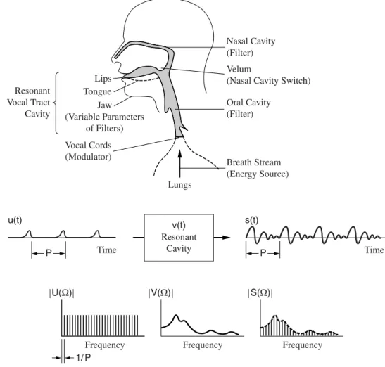
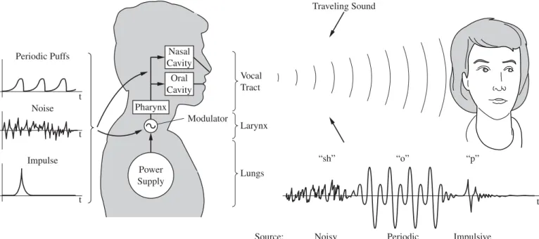
The larynx regulates airflow from the lungs and provides either an intermittent blowing or noisy source of airflow to a third group of organs, the vocal tract. The vocal tract consists of the oral, nasal, and pharyngeal cavities, which give "color" to the modulated airflow by spectrally shaping the source. Sound sources are idealized as periodic, impulsive or (white) noise and can occur in the larynx or vocal tract.
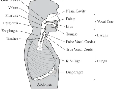
Anatomy and Physiology of Speech Production
- Lungs
- Larynx
- Vocal Tract
- Categorization of Sound by Source
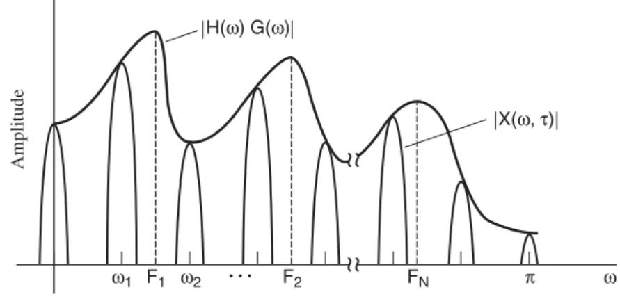
The resonant frequencies of the vocal tract are, in a speech science context, called formant frequencies or simply formants. The peaks of the spectrum of the vocal tract response correspond approximately to its formants. A formant corresponds to the vocal tract poles, while the harmonics arise from the periodicity of the glottal source.
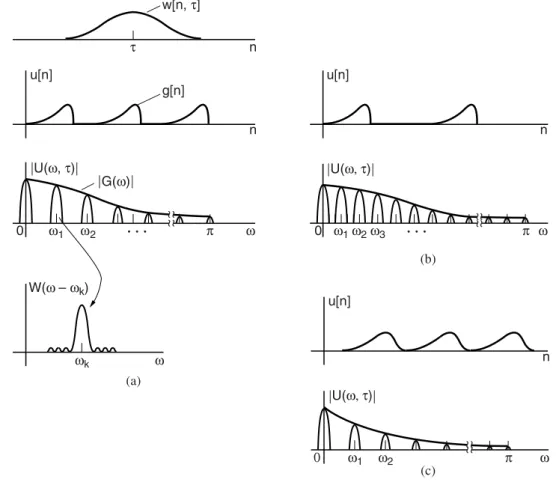
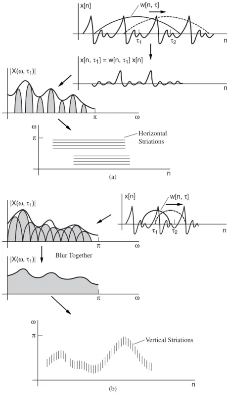
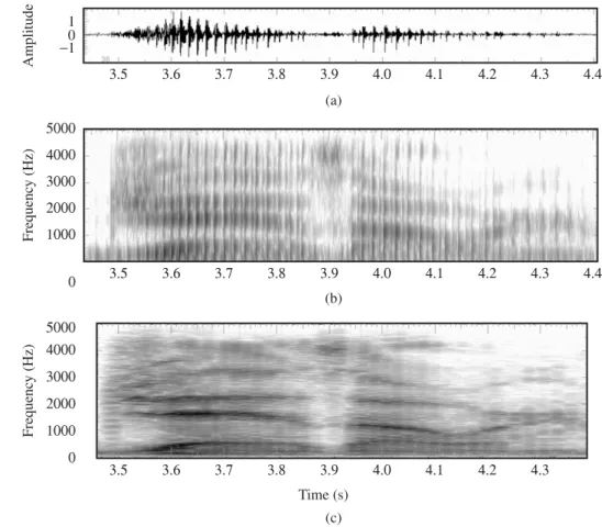
Spectrographic Analysis of Speech
Narrowband spectrogram—The difference between the narrowband and wideband spectrogram is the length of the window w[n, τ]. In our description of the narrowband and wideband spectrograms, we used the example of voiced speech. For plosives, the spectrogram reveals the general spectral structure of the sound as the window w[n, τ] slides over the signal.
Categorization of Speech Sounds
- Elements of a Language
- Vowels
- Nasals
- Fricatives
- Plosives
- Transitional Speech Sounds
The spectral nature of the sound is determined by the location of the tongue constriction. The narrowing can occur at the front, middle, or back of the oral canal (Figure 3.24). The fluids differ from the gliders in the formation of the constriction by the tongue; the tongue.
Prosody: The Melody of Speech
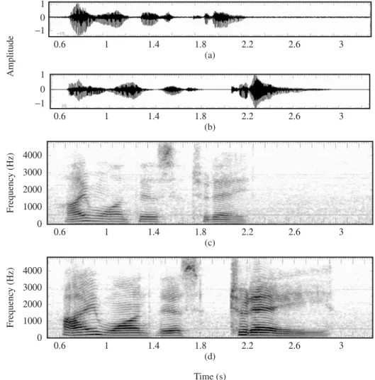
EXAMPLE 3.6 Figure 3.29 shows a comparison of the utterance "Please do this today," which is pronounced normally in the first case, while the word "today" is emphasized in the second. Feel your lungs constrict as you emphasize the word "today." The increase in lung contraction causes an increase in subglottal pressure. Another change in the emphasis of a sound is the increase in duration, as seen in the waveforms and spectrograms of the word "today" in Figure 3-29.
Speech Perception
- Acoustic Cues
- Models of Speech Perception
If /d/ is extracted in the word "do" and the delay between /d/ and /o/ is continuously increased, "do" will be perceived as "two" when the voice onset time exceeds approx. 25 ms [33 ]. For example, consider the phoneme /b/ in the word "be". The formant transition duration between /b/ and the following vowel /i/ is about 10 ms. We are now interested in the physiological correlates of these attributes, ie. the mechanism in the brain that registers the acoustic features that ultimately lead to the meaning of the message.
Summary
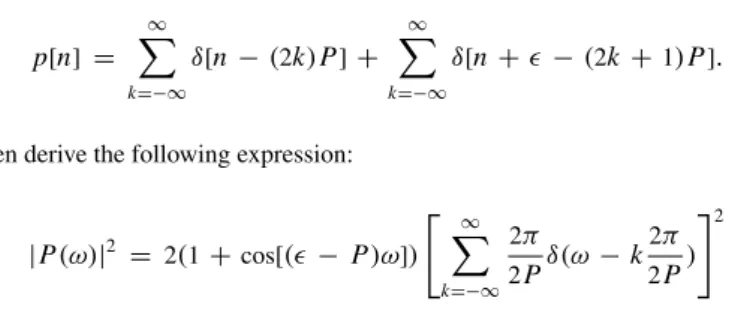
With this result, write the Fourier transform of the periodic glottal flow waveform[n], i.e. U (ω). b) Suppose, in a diplophonic condition, that no=P /2, where P is the glottal pitch period. Assume that the width of the window Fourier transform main lobe is less than 2πP, where P is the pitch period. Approximate the Fourier transform of the window by its main lobe only, that is, up to the first positive- and negative-frequency zero crossing.
Introduction
The idea of a vocal tract transfer function assumes that the vocal tract is linear and time invariant. More accurate models invoke a time-varying vocal tract and non-linear coupling between the vocal tract input, i.e. the glottal airflow velocity, and the pressure in the vocal tract resonant cavity. In Section 4.5, a simplified model of the non-linear interaction between the glottal source and a time-varying vocal tract is described.
Physics of Sound
- Basics
- The Wave Equation
The pressure increase in front of the wall moves like a chain reaction to the right. Alternatively, the wavelength is the distance traveled by the wave in one cycle of the vibration of the air particles. Newton's second law of motion states that the total force on the cube is the mass times the acceleration of the cube and is written as F =ma.

Uniform Tube Model
- Lossless Case
- Effect of Energy Loss
- Boundary Effects
- A Complete Model
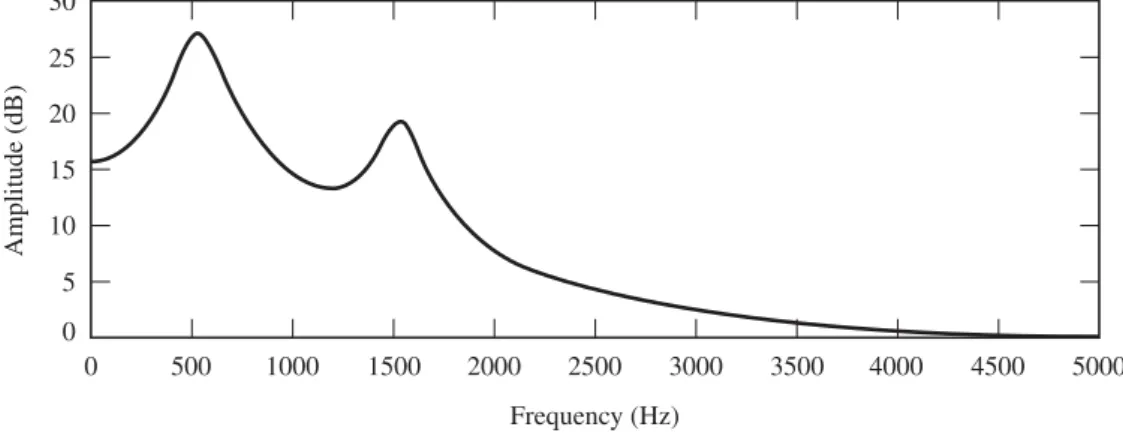
We write source as a function of frequency because we are ultimately interested in the frequency response of the uniform tube. Now consider the specific relationship between the volume velocity at the open end of the tube (the lips) and the volume velocity at the source (the glottis). The resulting frequency response Va()= U(1,)Ug() of the numerical simulation is shown in Figure 4.10a (pressure and velocity calculated at 96 samples in space along the xvariable) for a uniform tube with compliant walls and no other losses . ended in a zero pressure limit condition [26].
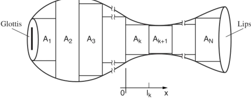
A Discrete-Time Model Based on Tube Concatenation
- Sound Propagation in the Concatenated Tube Model
- A Discrete-Time Realization
- Complete Discrete-Time Model
Similarly, uN(lN, t) = uL(t), which is the volume velocity at the exit of the lips. The flowchart in Figure 4.18a suggests, because of the discrete delay elements, that the concatenated tubes can be easily brought to discrete-time realization. G(z) is the z-transform of the glottal current input, g[n], over one cycle and may differ.
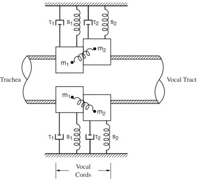
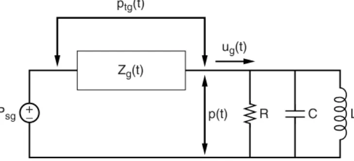
Vocal Fold/Vocal Tract Interaction
- A Model for Source/Tract Interaction
- Formant Frequency and Bandwidth Modulation
Only the first formant is included in Figure 4.22, because for higher formants the impedance of the vocal tract is negligible compared to that at the glottis. Numerical simulations, to describe, initially included multiple formants of the vocal tract and multiple subglottal resonances. The ripple has a frequency close to the first formant of the vocal tract, and the function f (t ) represents an amplitude modulation controlled by the glottal area function.
Summary
Assume the speech of sound = 350 m/s. d) Is it possible for a lossless connected tube model of the vocal tract to correspond to the spectrum of Figure 4.31. Use the radiation charge in Equation (4.24) and find the pressure in front of the lips at the mouth. Hz and the vocal tract is considered a single acoustic tube, which is the length of the vocal tract.
Introduction
This leads to a "pitch-synchronous" technique, based on the glottal closed phase, to separate the glottal flow waveform from the vocal tract impulse response. These methods do not constrain the glottal flow function to a maximum-phase bipolar model. Because the methods require us to view speech through a sliding window, we begin in Section 5.2 with a brief return to short time processing of speech.
Time-Dependent Processing
Next, in Section 5.7 we describe methods that generalize the analysis of an all-pole system to the estimation of a model transfer function consisting of poles and zeros.
All-Pole Modeling of Deterministic Signals
- Formulation
The coefficients are called the linear prediction coefficients, and their estimate is called linear prediction analysis[2]. Therefore, except for the times when ug[n] is non-zero, i.e. any pitch period, from equation (5.1) we can consider s[n] as a linear combination of previous values ofs[n], i.e., . We have assumed that the z-transform of the glottal airflow is approximated by two poles outside the unit circle, i.e. G(z) = (1−1βz)2.