distributed diagnosis of continuous systems

(1)

DISTRIBUTED DIAGNOSIS OF CONTINUOUS SYSTEMS: GLOBAL DIAGNOSIS THROUGH LOCAL ANALYSIS

By

Indranil Roychoudhury

Dissertation

Submitted to the Faculty of the Graduate School of Vanderbilt University

in partial fulllment of the requirements for the degree of

DOCTOR OF PHILOSOPHY in

Computer Science

August, 2009 Nashville, Tennessee

Approved:

Professor Gautam Biswas Professor Xenofon Koutsoukos

Professor Gabor Karsai Professor Sankaran Mahadevan

Professor Nilanjan Sarkar

(2)

(3)

To Ma, Baba, and Minu didi.

(4)

PREFACE

Early detection and isolation of faults is crucial for ensuring system safety and eciency. Online diagnosis schemes are usually integrated with fault adaptive control schemes to mitigate these fault eects, and avoid catastrophic consequences. These diagnosis approaches must be robust to uncertainties, such as sensor and process noise, to be eective in real world applications. Also, diagnosis schemes must address the drawbacks of centralized diagnosis schemes, such as large memory and computational requirements, single points of failure, and poor scalability. Finally, to be eective, fault diagnosis schemes must be capable of diagnosing dierent fault types, such as incipient (slow) and abrupt (fast) faults in system parameters.

This dissertation addresses the above problems by developing: (i) a unied qualitative diagnosis framework for incipient and abrupt faults in system parameters; (ii) a distributed, qualitative diagnosis approach, where each diagnoser generates globally correct diagnosis results without a centralized coordinator and communicates minimal measurement information and no partial diagnosis results with other diagnosers; (iii) a centralized Bayesian diagnosis scheme that combines our qualitative diagnosis approach with a Dynamic Bayesian network (DBN)-based diagnosis scheme; and (iv) a distributed DBN-based diagnosis scheme, where the global DBN is systematically factored into structurally observable independent DBN factors that are decoupled across time, so that the random variables in each DBN factor are conditionally independent of those in all other factors, given a subset of communicated measurements that are converted into system inputs. This allows the implementation of the combined qualitative and DBN-based diagnosis scheme on each DBN factor, which operate independently with a minimal number of shared measurements to generate globally correct diagnosis results locally without a centralized coordinator, and without communicating any partial diagnosis results with other diagnosers. The correctness and eectiveness of these diagnosis approaches is demonstrated by applying the qualitative diagnosis approaches to the Advanced Water Recovery System developed at NASA Johnson Space Center; and the DBN-based diagnosis schemes to a complex, twelfth-order electrical system.

(5)

ACKNOWLEDGMENTS

I am indebted to my advisors, Professors Gautam Biswas and Xenofon Koutsoukos, for their in- valuable comments, critiques, and guidance that ensured the completion of my research and this dissertation. I would also like to thank the remaining members of the committee, Professors Gabor Karsai, Sankaran Mahadevan, and Nilanjan Sarkar, for their insight on the research presented in this dissertation.

I owe thanks to Matthew Daigle, Nagabhushan Mahadevan, Manish Kushwaha, Joe Porter, Ashraf Tantawy, Chetan Kulkarni, Jian Wu and Eric Manders for the numerous fruitful discussions and brain-storming sessions that helped improve the quality of this work. I would also take this opportunity to express my gratitude to other past and present members of our research group, and friends outside this group, who made my stay at Vanderbilt enjoyable and fun. Of course, this dissertation would have never materialized without the undying support of my family, and I dedicate this work to them.

The two summers I have spent at NASA Ames Research Center working on the Advanced Di- agnostics and Prognostics Testbed (ADAPT) have been very rewarding, and I would like thank the members of the ADAPT Team, Ann Patterson-Hine, Scott Poll, Adam Sweet, Joe Camisa, David Nishikawa, David Hall, Serge Yentus, Charles Lee, Christian Neukom, John Ossenfort, and David Garcia for the same.

This work was supported in part by the National Science Foundation under Grants CNS-0347440, CNS-0452067, CNS-0615214, and NSF ITR grant CCR-0225610, and National Aeronautics and Space Administration under grants NRA NNX07AD12A, NASA USRA 08020-013, NASA SGER 0208799, and NASA-ALS NCC 9-159.

(6)

TABLE OF CONTENTS

Page

PREFACE . . . iv

ACKNOWLEDGMENTS . . . v

LIST OF TABLES . . . viii

LIST OF FIGURES . . . ix

Chapter I. INTRODUCTION . . . 1

Motivation . . . 1

Research Contributions . . . 3

Organization of Dissertation . . . 6

II. RELATED WORK IN MODEL-BASED DIAGNOSIS OF DYNAMIC SYSTEMS . . . 9

A Taxonomy of Faults . . . 9

A Taxonomy of Model-Based Fault Diagnosis Approaches . . . 11

Robust Model-Based Fault Diagnosis Approaches . . . 14

Discrete-Event Systems Diagnosis . . . 16

Discussion . . . 20

Diagnosis Using Qualitative Models . . . 21

Discussion . . . 23

Analytical Redundancy Relations-Based Diagnosis Scheme . . . 24

Discussion . . . 26

Probabilistic Diagnosis Schemes . . . 27

Model-based Diagnosis using Bayesian Networks . . . 30

Model-Based Diagnosis Using Dynamic Bayesian Networks . . . 33

Discussion . . . 42

Summary . . . 44

III. THE TRANSCEND DIAGNOSIS APPROACH . . . 47

Modeling for Diagnosis . . . 48

Bond Graphs . . . 48

Deriving State Space Equations from Bond Graphs . . . 53

Modeling Abrupt Faults . . . 55

Temporal Causal Graphs . . . 56

Deriving Temporal Causal Graphs from Bond Graphs . . . 57

Tracking and Fault Detection . . . 59

Tracking . . . 59

Fault Detection . . . 59

Qualitative Fault Isolation . . . 60

Symbol Generation . . . 61

Hypothesis Generation . . . 62

Hypothesis Renement . . . 63

Fault Identication . . . 65

Extending Transcend To Include Diagnosis of Incipient Faults . . . 66

Modeling Incipient Faults . . . 67

(7)

Extending Hypothesis Generation . . . 67

Extending Fault Signature Derivation . . . 68

Diagnosability Analysis . . . 69

Summary . . . 70

IV. DISTRIBUTED QUALITATIVE DIAGNOSIS OF CONTINUOUS SYSTEMS . . . 72

The Distributed Diagnosis Approach . . . 73

Formulating the Design Problem for Distributed Diagnosis . . . 75

Designing the Distributed Diagnosers . . . 79

Implementing Distributed Qualitative Isolation . . . 79

Designing Diagnosers for a Partitioned System . . . 80

Designing Diagnosers for an Unpartitioned System . . . 82

Case Study: The Advanced Water Recovery System . . . 84

System Overview . . . 84

Diagnoser Design Experiments . . . 88

Distributed Fault Isolation . . . 93

Summary and Conclusions . . . 95

V. CENTRALIZED BAYESIAN DIAGNOSIS OF COMPLEX SYSTEMS . . . 99

Deriving Dynamic Bayesian Networks For Complex Systems . . . 101

Fault Detection and Qualitative Fault Isolation . . . 105

Quantitative Fault Isolation and Identication . . . 106

Approach 1: Including Faulty Parameter as State Variable . . . 111

Approach 2: Including Fault Magnitude or Slope as State Variable . . . 115

Approach 3: Computing Maximum Likelihood Estimate of Fault Parameter . . . 119

Discussion . . . 122

Structural Observability . . . 124

Case Study: Twelfth-order Electrical Circuit . . . 130

Discussion and Summary . . . 138

VI. DISTRIBUTED BAYESIAN DIAGNOSIS OF CONTINUOUS SYSTEMS . . . 141

Formulating the Design Problem for Distributed Diagnosis . . . 142

Designing the Distributed Diagnosers . . . 146

Implementing the Individual Distributed Diagnosers . . . 152

Experimental Results for Distributed State Estimation Using DBN-Fs . . . 154

Case Study 2: Diagnosis Experiments on the Twelfth-order Electrical Circuit . . . 155

Distributed Diagnoser Design . . . 156

Distributed Diagnosis Experimental Results . . . 157

Discussion and Summary . . . 167

VII. CONCLUSIONS . . . 170

Future Directions . . . 172

Appendix REFERENCES . . . 174

(8)

LIST OF TABLES

Table Page

1 Summary of Related Work . . . 46

2 Fault signatures from abrupt faults in the two-tank system . . . 64

3 Selected fault signatures for the two-tank system . . . 69

4 Six-tank measurements available for diagnosis . . . 76

5 Fault signatures from tanks 1 and 2 of the six-tank system . . . 77

6 Fault signatures for the six-tank system example . . . 80

7 Measurements and faults chosen for the experiments . . . 89

8 Results for Experiments 1-A, 1-B, and 1-C . . . 90

9 Results for Experiment 2-A (17 measurements) . . . 91

10 Results for Experiment 2-B (14 measurements) . . . 91

11 Results for Experiment 2-C (16 measurements) . . . 93

12 Some fault signatures for the AWRS diagnosis experiment . . . 93

13 Diagnosis results for 20% abrupt fault RO.R^+a_pipe at t_f = 21000seconds. . . 94

14 Selected fault signatures for the two-tank system . . . 113

15 Selected fault signatures for the electrical circuit . . . 133

16 Results of Centralized Diagnosis Experiments on the Twelfth-Order Electrical Circuit . 138 17 Average mean squared error and standard deviation over all state variables across10runs 155 18 Time taken for particle lter to complete estimation . . . 155

19 Fault Signatures for Diagnoser D1 . . . 156

20 Fault Signatures for Diagnoser D2 . . . 157

21 Results of Distributed Diagnosis Experiments on the Twelfth-Order Electrical Circuit with Particles Used Proportional to The Total Number of States per Factor . . . 164

22 Results of Distributed Diagnosis Experiments on the Twelfth-Order Electrical Circuit with500 Particles Used per Factor . . . 164

23 Results of Distributed Diagnosis Experiments on the Twelfth-Order Electrical Circuit with750 Particles Used per Factor . . . 164

24 Results of Distributed Diagnosis Experiments on the Twelfth-Order Electrical Circuit with1000Particles Used per Factor . . . 165

(9)

LIST OF FIGURES

Figure Page

1 Scope of this dissertation with respect to the types of faults we diagnose. . . 10

2 The architecture of a generic model-based diagnosis approach. . . 13

3 Schematic of a two tank system with quantized states. . . 17

4 Quantized state-space of the two-tank system. Grey arrows depict normal transitions, the black arrow shows an unobservable faulty transition. . . 17

5 A FSM for the two-tank system. . . 18

6 Signed digraph for a simple tank system. . . 22

7 Architecture of a generic model-based diagnosis approach where detection and isolation of faults are combined. . . 24

8 Schematic of a one tank system. . . 29

9 A Simplied Bayesian Network for the two-tank system. . . 32

10 Dynamic Bayesian network of a two-tank system. . . 34

11 Computational architecture of the Transcend fault diagnosis approach. . . 48

12 The example nonlinear two-tank system. . . 50

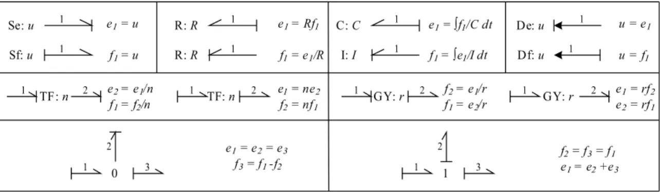
13 Possible causal assignments and corresponding constituent equations of bond graph elements. . . 51

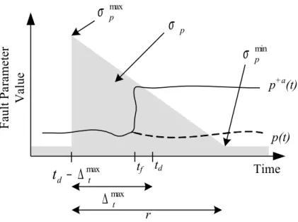
14 Abrupt fault prole. . . 56

15 Generating temporal causal graphs from bond graphs. . . 57

16 Temporal causal graph of the two-tank system. . . 58

17 Symbolic abstractions of measurement deviations (adapted from [1]). . . 61

18 Block diagram of the fault identication procedure. . . 66

19 Incipient fault prole. . . 67

20 Architecture of the distributed qualitative fault diagnosis approach. . . 74

21 The six-tank system. . . 75

22 Bond graph model of the six-tank system. . . 75

23 Temporal causal graph for the six-tank system. . . 76

24 Schematic of the Advanced Water Recovery System. . . 85

25 Bond graph model of the Biological Water Processor. . . 86

26 Bond graph model of the Reverse Osmosis Subsystem. . . 87

27 Bond graph model of the Air Evaporation System. . . 88

28 Experimental observations. . . 96

29 The diagnosis architecture. . . 100

30 Two tank TCG containing displacement variablesq2 andq7. . . 102

31 Simplied Temporal Causal Graph of the two-tank system. . . 103

32 Dynamic Bayesian network of a two-tank system. . . 103

33 Computational Architecture of Quant-FHRI. . . 107

34 Prole of standard for our particle ltering-based fault identication. . . 110

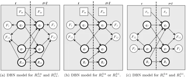
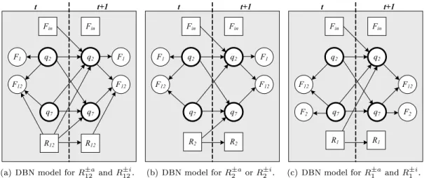
35 Single DBN model for both abrupt and incipient faults in the same parameter in Quant- FHRI Approach 1. . . 111

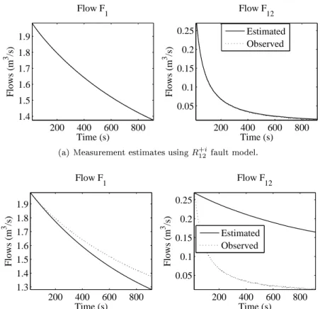
36 Results of diagnosing faultR⁺ⁱ₁₂ using Quant-FHRI Approach 1. . . 114

37 Estimated slope of the true faultR⁺ⁱ₁₂ using Quant-FHRI Approach 1. . . 114

38 Results of diagnosing faultR^+a₁ using Quant-FHRI Approach 1. . . 115

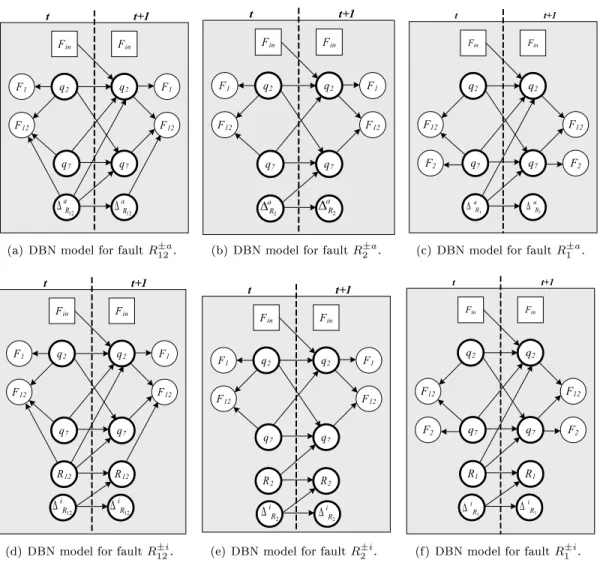
39 Separate DBN models for abrupt and incipient faults in the same parameter in Quant- FHRI Approach 2. . . 116

41 Estimated values of the true faultR⁺ⁱ₁₂ and fault slope∆ⁱ_R 12 using Quant-FHRI Approach 2. . . 118

(10)

43 Single DBN model for both abrupt and incipient faults in the same parameter in Quant-

FHRI Approach 3. . . 120

45 Estimation results of R₁₂ using Quant-FHRI Approach 3. . . 122

48 Junction Structure. . . 127

49 Electrical circuit models. . . 131

50 DBN model of the electrical circuit. . . 132

51 Detection ofC₂^−a fault through tracking system behavior using nominal DBN model. . . 133

52 Tracking faulty system behavior using theC₂^±i/C₂^±a DBN fault model. . . 134

53 Tracking faulty system behavior using theR^±i₂ /R^±a₂ DBN fault model. . . 135

54 Sum of mean squared estimation errors obtained byC2 andR2 DBN fault models. . . . 136

55 Estimate of C2 obtained using theC2 DBN fault model. . . 136

56 Detection ofL⁻ⁱ₃ fault through tracking system behavior using nominal DBN model. . . 137

57 Estimate of L3 obtained using theL3 DBN fault model. . . 137

58 Parameter identication results for electrical circuit example. . . 138

59 The distributed diagnosis architecture. . . 142

60 Models of the tenth-order electrical system. . . 143

61 Factorings of the electrical system DBN. . . 145

62 Four-factored bond graph of the electrical circuit with imposed derivative causality. . . 146

63 Three-factored bond graph of the electrical circuit with imposed derivative causality. . . 151

64 Two-factored bond graph of the electrical circuit with imposed derivative causality. . . . 151

65 Two-factored DBN for the twelfth-order electrical circuit. . . 155

66 Two-Factored bond graph of the twelfth-order electrical circuit with imposed derivative causality. . . 157

67 DBN-F Fault models for distributed diagnosis experiments using the Quant-FHRI approach 1. . . 158

68 Detection ofC₂^−a fault by diagnoserD1. . . 159

69 Tracking observations in the presence of C₂^−a fault by diagnoserD2. . . 160

70 Tracking faulty system behavior using theC₂^±i/C₂^±a DBN-F fault model. . . 161

71 Tracking faulty system behavior using theR^±i₂ /R^±a₂ DBN-F fault model. . . 162

72 Sum of mean squared estimation errors obtained byC₂ andR₂ DBN-F fault models. . . 163

73 Estimate of C₂ obtained using theC₂ DBN-F fault model. . . 163

74 Detection ofL⁻ⁱ₃ fault by diagnoserD₁. . . 164

75 Tracking observations in the presence of L⁻ⁱ₃ fault by diagnoserD₂. . . 165

76 Estimate of L₃ obtained using theL₃ DBN-F fault model. . . 165

77 Parameter identication results for electrical circuit example. . . 166

78 % MAE and convergence time of distributed Bayesian experiments for dierent numbers of particles. . . 166

(11)

CHAPTER I

INTRODUCTION

Motivation

Modern day engineered systems are a product of careful design and manufacturing, and undergo rigorous testing and validation before deployment. This reduces the likelihood of system failures, but degradation and faults in system components still occur due to wear and tear from sustained operations. Unlikely events and unanticipated situations can also create faults. Early detection and isolation of faults is the key to maintaining system performance, ensuring system safety, and increasing system life. Traditionally, the fault diagnosis task has been performed oine during maintenance operations, using test results and alarm signals to isolate faults in system components.

For present-day, safety-and-mission critical systems, it is imperative to monitor system behavior and performance online, i.e., during operation, so that system control and operation can adapt to changes and avoid catastrophic failures.

The process of fault diagnosis consists of detection, isolation, and identication of faults [2].

Fault detection typically produces a binary decision that determines whether the observed system behavior has deviated from the expected nominal behavior. Fault isolation involves determination of the cause of the fault, and is sometimes called root cause analysis. Fault identication is the task of determining the extent or magnitude of the fault. We consider a fault to be a change in the system which causes the system's behavior to deviate from the expected nominal behavior. Faults manifest at dierent locations, e.g., in the sensors, actuators, or plants. These faults may manifest at very fast rates (called abrupt faults) or they may be gradual (called incipient faults). In some cases, they may cause unwanted changes in the system structure. Hence, fault diagnosis schemes must be generally applicable and apply to dierent kinds of faults.

Fault diagnosis approaches can be broadly classied as model-free and model-based methods [2].

Model-based approaches are considered to be more general than model-free approaches that are mostly based on expert knowledge and data-driven methods. Model-based approaches posses prov- able properties, such as detectability and isolability of sets of faults. Typically there is a clear separation between the particular model and the reasoning algorithm used in model-based diagnosis approaches. Again, in contrast to model-free approaches, this contributes to more general and

(12)

the system operating ranges and modes of operation, and any change in the system components or operating ranges usually require the recalibration of the parameters and thresholds used in the detection and isolation scheme. The generation of appropriate system models to support diagnosis, however, can be a challenge, since, real-world systems encompass multiple domains, such as the hydraulic, electrical, and mechanical domains. Their behaviors can contain sharp nonlinearities, and it may be dicult to capture all possible interactions between components of the system, and between the system and the environment. Moreover, the system models have to be built at the correct level of abstraction, balancing the details needed in the model to make the system diagnosable, while keeping the model complexity low, so as to not aect the performance of online diagnosis.

In the real world, uncertainties caused by measurement and process noise, and modeling abstractions and errors are unavoidable. Therefore, eective fault diagnosis schemes must be robust to these uncertainties, and generate correct diagnosis of faults in their presence. Probabilistic reasoning techniques are well suited for this purpose and are based on an intuitive and theoretically sound mathematical foundation which generates consistent diagnostic results under uncertainties, and usually require the generation of probabilistic system models, such as Dynamic Bayesian Net- works (DBNs), to capture the uncertainties in the systems to be diagnosed [3]. Once generated, standard Bayesian inference approaches are applied on these probabilistic models to diagnose faults correctly in the presence of uncertainties. However, exact computation of probabilities for systems, barring a few restricted cases, is computationally exponential, and hence, approximate methods for computing these probabilities have to be applied. But, these approximate Bayesian inference schemes can be computationally very expensive for large systems, and may suer from convergence issues [3, 4].

High costs, such as memory and computational requirements, plague most centralized model- based diagnosis schemes (probabilistic, or otherwise), since these schemes involve one monolithic diagnoser that operates on a global system model and requires all available system measurements for diagnosis [2,5]. The computational expense can be reduced by distributing the diagnosis task into subtasks that can be executed on separate processors. Therefore, distributed diagnosis approaches t well with present day embedded systems architectures, where each subsystem has associated local processors, memory, and sensors for monitoring and control of that subsystem, e.g., electronic control units in aircrafts. In addition to improving computational eciency, distributed diagnosis schemes also reduce the high costs of shielding and protection of the cables usually incurred to transmit measurements to a centralized computer while maintaining signal quality, especially in harsh environment. Furthermore, distribution of the diagnosis task addresses other issues of

(13)

centralized diagnosis schemes, such as single points of failure, and poor scalability. In centralized diagnosis schemes, a glitch or failure in the diagnosis unit may disable the entire diagnosis system.

Distributed diagnosis approaches do not have any such single point of failure. Further, centralized diagnosis schemes scale poorly, since changes in the system conguration and components may cause signicant changes in the system's dynamic behavior, requiring the diagnoser to be redesigned.

Again this drawback can be addressed by distributing the diagnosis task.

Research Contributions

To address the aforementioned challenges in model-based diagnosis of real-world systems, this dissertation develops a distributed, probabilistic, model-based approach for the accurate diagnosis of incipient and abrupt faults in a unied framework, in the presence of uncertainties, such as sensor noise and process disturbances. By distributing the diagnosis task into smaller subtasks, we improve the computational eciency of our diagnosis approach. We further improve the computational e- ciency and scalability of our diagnosis approach by combining a qualitative diagnosis approach with a quantitative Bayesian state estimation scheme.

Incipient and abrupt faults are classications of parametric faults, which are characterized by unwanted changes in system parameters. Incipient faults are modeled as slow drifts in system parameter values caused by wear and tear in system components, such as degradation in the stator windings or bearings in induction motors [6] and gradual blockage in pipes in hydraulic or chemical systems due to the accumulation of sediments. Abrupt faults represent faults that are caused by unwanted changes, where the rate of change in system parameter is much faster than the dynamics of the system, or rate of sampling of system measurements. Hence, abrupt faults are modeled as step changes in the parameter values. Examples of abrupt faults include a sudden (partial or complete) blockage in a pipe carrying uid, or a bias that develops in a sensor. Since both abrupt and incipient faults are common in real-world engineering systems, our comprehensive diagnosis scheme applies to both these types of faults in a unied framework.

The specic research contributions of this thesis are listed below.

1. Qualitative diagnosis of incipient and abrupt faults in a unied framework: We extend the Transcend qualitative diagnosis scheme [7,8] to allow for qualitative diagnosis of both incipient and abrupt faults in a unied framework. The qualitative Transcend diagnosis approach was originally designed for the diagnosis of abrupt faults. The isolation of abrupt

(14)

in measurements from nominal behavior are matched against qualitative predictions of faulty behavior, known as fault signatures, to isolate faults. We extend the diagnosis scheme to include the detection and isolation of incipient faults.

2. Distributed qualitative diagnosis of incipient and abrupt faults: We develop a distributed Transcend-based qualitative diagnosis scheme for continuous dynamic systems.

Most of the previous work in distributed diagnosis has been developed for discrete event system models [9, 10], but these methods do not scale up for complex continuous systems [11]. Our distributed diagnosis approach designs a multiple diagnoser solution that generates globally correct diagnosis results by local analysis without a centralized coordinator, with no exchange of partial diagnosis results amongst the diagnosers, and with minimal sharing of measurements. We propose two approaches for designing the distributed qualitative diagnosers. The rst algorithm assumes the subsystem structure is known and constructs a local diagnoser for each subsystem. The second algorithm creates a partition structure and local diagnosers simultaneously. The absence of a centralized coordinator ensures that our distributed diagnosis scheme does not have a single point of failure. Moreover, because a distributed diagnoser does not depend on the partial diagnosis results of other diagnosers for its own diagnosis, the failure of individual diagnosers do not aect the performance of the other diagnosers. Hence, our distributed diagnosis scheme degrades gracefully as one or more distributed diagnosers fail. Also, in our distributed diagnosis scheme, the diagnosis task is distributed amongst the dierent distributed diagnosers, and hence, this distributed scheme is computationally less expensive than its centralized counterpart.

3. Ecient Bayesian diagnosis of incipient and abrupt faults: We combine the Tran- scend qualitative fault isolation with a DBN-based state and parameter estimation scheme to develop an ecient probabilistic approach for diagnosis of both incipient and abrupt faults in continuous dynamic systems using DBNs to explicitly model the system dynamics and uncertainties. To accommodate nonlinearities, and non-Gaussian distributions, we employ a particle ltering-based state estimation scheme for diagnosis [12]. We use particle lters to ensure that our Bayesian diagnosis scheme is generally applicable to complex nonlinear systems, with non- Gaussian probability distributions. However, particle ltering-based fault diagnosis schemes suer from the sample impoverishment problem [4, 13]. We develop a solution to this problem, and describe three dierent fault identication approaches to estimate the value of the faulty parameter based on the observed measurements, and isolate the true fault. The use of

(15)

Bayesian estimation ensures robustness to measurement and process noise, and provides more precise diagnosis results than our qualitative Transcend-based diagnosis scheme. However, the Bayesian state estimation scheme can be computationally expensive for large systems. We improve the eciency of this Bayesian diagnosis scheme by integrating it with our extended qualitative Transcend diagnosis scheme. The eciency gain is obtained by rst using the qualitative diagnosis scheme to rene the possible fault hypotheses to a tractable number, and then invoking multiple DBN-based ltering schemes for the reduced fault hypothesis set.

4. Distributed Bayesian diagnosis of incipient and abrupt faults: We develop a distributed combined qualitative and Bayesian diagnosis scheme that further improves the e- ciency of our centralized diagnosis scheme. The basis of our distributed Bayesian diagnosis scheme is the factoring of the system DBN model into multiple, non-overlapping DBN factors, such that each random variable in a DBN factor is conditionally independent of random variables in all other DBN factors given the measurements communicated between these factors. Our DBN factoring scheme is based on computing some state variables in the system as algebraic functions of measurements (considered to be system inputs), which allows the replacement of the across-time links between these state variables with new intra-time links from the measurements to the state variables. If sucient number of across-time links are removed, we can factor the system DBN into DBN factors such that the random variables in each generated factor is conditionally independent from those in any other factor, given the measurements that were used to compute some state variables. It is well-known that the state variables of a system can be estimated from the system measurements only if the system is observable. We ensure that each factor is observable based on the analysis of structural observability properties of the system's bond graph model and its component parts [14, 15]. We analyze the structural observability properties of the system to ensure that each DBN factor represents a structurally observable subsystem, and together all the DBN factors retain the structural observability properties of the global system. Once the global DBN is factored, the conditional independence of the random variables in each DBN factor allow the implementation of Bayesian estimation schemes on each DBN factor independently. For our distributed Bayesian diagnosis scheme, we apply our combined qualitative-quantitative diagnosis scheme on each DBN factor instead of the global system DBN. Previous work in factored estimation schemes, such as the Boyen-Koller algorithm, presented in [16], creates the individual factors by eliminating causal links between weakly interacting subsystems. Therefore, the belief state

(16)

derived from the individual factors is an approximation of the true belief state. The error in this approximation is bounded, but these bounds may not be suciently precise for online monitoring of mission-critical systems. The novelty of our factoring scheme lies in the fact that the DBN factors together preserve the overall system dynamics in the factored form, and there is no approximation involved in the factored belief state.

5. Experimental studies. We apply our distributed qualitative diagnosis approaches to a complex, real-world system, the Advanced Water Recovery System, which was designed and built at the NASA Johnson Space Center to convert wastewater into potable water for long duration manned missions [17]. Our centralized and distributed Bayesian diagnosis schemes are applied to a complex, twelfth-order electrical circuit, with highly oscillatory behavior. The use of Bayesian diagnosis schemes result in correct and precise diagnosis results in the presence of noisy sensors, while our distributed diagnosis schemes address the drawbacks of centralized diagnosis approaches, especially by improving the computational eciency when compared to the centralized schemes.

Our distributed approach assumes faults are persistent, abrupt or incipient, and parametric. We assume that the faults are non-catastrophic, i.e., the system still can operated, albeit in a degraded state, after fault occurrence. We make the single fault assumption since simultaneous multiple fault occurrences are much less likely.

Organization of Dissertation

This dissertation is organized as follows. Chapter II presents related work in model-based diagnosis of continuous systems. We start with a taxonomy of faults and fault diagnosis approaches. Then we present and compare dierent model-based diagnosis schemes for dynamic systems, and how these dierent schemes handle uncertainties. Specically, we describe dierent diagnosis approaches, such as discrete-event systems approaches, qualitative diagnosis schemes, analytical redundancy relations- based diagnosis approaches, and probabilistic model-based diagnosis schemes. We conclude this chapter by presenting our diagnosis approaches in context of the related work.

Chapter III starts with the necessary background on the Transcend qualitative diagnosis scheme, and extends it to the combined diagnosis of incipient and abrupt faults. We begin by presenting the modeling paradigms used in Transcend, i.e., bond graphs [18] and temporal causal graphs (TCGs) [7], and then describe, in detail, the dierent steps of the Transcend diagnosis scheme. Then, we present our extensions to Transcend for the diagnosis of incipient faults.

(17)

Specically, we describe how we have extended the Transcend fault signature generation scheme to generate fault signatures for incipient faults. This allows for seamless integration of incipient and abrupt fault diagnosis in Transcend. Finally, we present an analysis of the diagnosability properties of the Transcend qualitative diagnosis scheme for the unied qualitative diagnosis of incipient and abrupt faults.

Chapter IV describes our distributed qualitative scheme for diagnosis abrupt and incipient faults.

First, we present our distributed diagnosis architecture, where each distributed diagnosis is essentially a Transcend diagnoser that uses a subset of observations to diagnose a subset of faults.

Through the careful design of these distributed diagnosers, we guarantee that each distributed diagnoser will generate globally correct diagnosis results through local analysis, without a centralized coordinator, and no exchange of partial diagnosis results, but through the communication of minimal number of measurement information. Two approaches for designing the distributed qualitative diagnosers are presented. In the rst diagnoser design approach, we assume knowledge of subsystem structure, especially the measurements and faults that belong to each subsystem, and based on this information, we design a local diagnoser for each subsystem such that it required minimal number of additional external measurements to globally diagnose all the faults assigned to that subsystem. In the second approach, we assume no prior partitioning information. Instead, we generate the maximal number of distributed diagnosers, such that, each local diagnoser can operate independently without sharing any measurements to generate globally correct diagnosis results. The formulation of the diagnoser design problems and the algorithms for designing these distributed diagnosers are described in the next two sections. This is followed by a set of studies that demonstrate the usefulness of this distributed diagnosis approach. We then present a case study for a real-world engineering system.

We verify the correctness and ecacy of the dierent diagnosis approaches and the DBN factoring scheme by applying them to the Advanced Water Recovery System, developed at the NASA Johnson Space Center, a real-world large engineering system.

Chapter V presents our centralized Bayesian scheme for diagnosing abrupt and incipient faults in continuous systems, where we combine the qualitative Transcend fault isolation scheme with a DBN-based quantitative fault hypothesis renement and identication approach. First, we present the computational architecture of our diagnosis approach, and then describe the procedure for systematically deriving the DBNs for nominal and faulty system behavior from the system bond graph.

The following section presents our centralized diagnosis approach, which includes detection, isolation, and identication of the fault hypotheses using a particle ltering-based state estimation scheme.

(18)

Use of this approach requires addressing the sample impoverishment problem, as discussed in the following section. This is followed by a set of experimental results that demonstrate the ecacy of our diagnosis scheme. We conclude this chapter with a discussion of the contributions in this work.

Chapter VI presents our distributed Bayesian approach for diagnosing incipient and abrupt faults. We start by presenting our distributed diagnosis architecture. Then we formulate the diagnoser design problem. The main idea is to factor the system's global DBN into conditionally independent DBN factor, such that each DBN factor is structurally observable, and apply the combined qualitative-Bayesian diagnosis scheme on each DBN factor independently. We present our diagnoser design approach based on factoring the system DBN into structurally observable DBN factors in the following section. The next section provides proof that the design of our distributed diagnosers ensures that our distributed diagnosis properties of generating globally correct diagnosis through local analysis is satised. We then present some experimental results to demonstrate the eectiveness of our factored estimation and distributed diagnosis scheme.

Chapter VII summarizes the contributions of this dissertation, and presents some conclusions.

We also describe the current limitations of our approaches, and identify future directions of work to improve the current research.

(19)

CHAPTER II

RELATED WORK IN MODEL-BASED DIAGNOSIS OF DYNAMIC SYSTEMS

Timely detection and isolation of faults is very important for ecient and safe performance of engineering systems. For safety critical systems, such as aircraft, a fault in its component, if it goes undetected, may have serious consequences in terms of the system's operation, and cause loss of life and property. A potentially harmless fault in a computer network can hinder the productivity of oce sta, and result in monetary losses and unexpected delays. Given the varied nature of faults, and the adverse eects they can have on system operation, the task of accurate and timely diagnosis of system faults in complex dynamic systems presents a number of important and interesting research challenges. In this chapter, we provide a taxonomy of faults and present several classical model-based diagnosis approaches that have been developed for the detection and isolation of faults in dynamic systems.

A Taxonomy of Faults

Faults are undesired changes that cause deviations in expected system behavior, which then aect system performance [2, 7]. In this research, we dierentiate faults from complete failures of the system. We assume that faults cause degradation in system performance, but may not result in complete loss of system functionality. As an example, a short-circuit in a battery that causes the battery to explode is considered a failure, and hence, beyond the scope of this dissertation. However, the gradual or an abrupt decrease in the battery's charge storage capacity is considered a fault, since the battery can still operate in a degraded manner. We adopt the terminology used in the domain of fault detection and isolation [2, 19, 20] to present the dierent concepts in the remainder of this chapter.

Denition 1 (Fault). A fault is an unexpected change in the plant or its instrumentation that causes the system to deviate from its nominal behavior.

Faults can be classied based on how they are modeled, their temporal prole, and their location, as shown below.

1. Fault Model: Based on how they are modeled, faults can be classied as additive, parametric,

(20)

SensorActuatorPlant

Incipient Intermittent Abrupt

Additive Discrete

Parametric Abrurur pupu t Inncipient Parametric

Plant

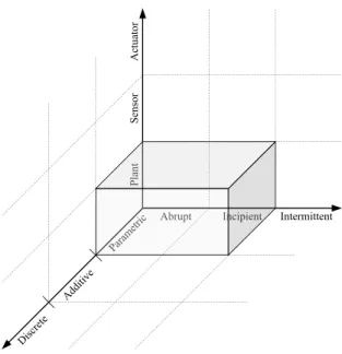
Figure 1: Scope of this dissertation with respect to the types of faults we diagnose.

zero. Additive fault eects are decoupled from the system dynamics, therefore, they can be studied by analyzing changes in the system input-output relations without changing the basic system dynamics model. Examples of additive faults include sensor faults (if the sensor measurements are not part of the control loop), small leaks in a system, and changes to the plant loads. A discrete fault causes a change in the system structure or topology. Examples of discrete faults include broken wires and unexpected changes in a system's conguration.

Parametric faults result in changes to the system parameters, and hence, these faults directly impact the system dynamics. Therefore, fault eects cannot be analyzed by decoupling them from the nominal system dynamics. In other words, parametric faults directly aect the system's dynamic behavior and one has to analyze the nominal system and fault dynamics simultaneously to isolate these faults. Examples of parametric faults include changes in the parameter values of physical processes in the system, such as, the energy storage elements or the dissipative elements.

2. Temporal prole: The temporal prole of a fault is linked to the persistence of a fault's eects. Persistent faults do not disappear once they have occurred. On the other hand, intermittent faults manifest for some time, and then their eects cease to perturb the system dynamics. Intermittent faults typically appear and disappear at random intervals. Persistent faults can be further categorized as abrupt or incipient. Abrupt faults cause changes in parameter values that occur at a rate much faster than the nominal system dynamics. Abrupt

(21)

parametric faults are usually modeled as step-changes in component parameter values. In contrast, incipient faults develop slowly over time, and the change in fault parameter value is dened by a slow temporal function.

3. Fault location: Based on where faults are located in the system, they can be sensor, actuator and plant faults. While sensor faults are attributed to measurement devices, and characterized by discrepancies between the actual values of plant variables and the values reported by the instrumentation system, actuator faults are located at system inputs, and plant faults are characterized by faults in the system parameters.

In summary, a fault is completely dened by its fault model, temporal prole, and location. For example, a sensor bias fault is characterized as an additive, (persistent) abrupt, sensor fault. Simi- larly, some of the common failures in electric induction motors are dened as parametric, (persistent) incipient, plant faults.

As shown in Fig. 1, this dissertation research aims at diagnosing abrupt and incipient parametric plant faults in continuous dynamic systems. Faults in sensors and actuators, as well as discrete faults are beyond the scope of this dissertation.

A Taxonomy of Model-Based Fault Diagnosis Approaches

The task of fault diagnosis includes fault detection, fault isolation, and fault identication, as described below:

1. Fault Detection: Fault detection comprises of methods that produce binary decisions as to whether the deviation in system behavior from nominal is attributed to a fault in the system or not.

2. Fault Isolation: Fault isolation refers to schemes that determine the component or subsystem malfunction that explains the observed discrepancies in system behavior.

3. Fault Identication: Fault identication is the task of determining the magnitude or extent of the fault. For parametric faults, fault identication involves estimating the amount of deviation in an abrupt fault, or the rate at which an incipient fault parameter changes over time.

A number of fault diagnosis approaches have been developed by researchers and practitioners [7,

(22)

relationship between the observed symptoms and the faults. This prior domain knowledge may be derived from rst principles, domain-theoretic understanding of the system, such as physical system models derived using physical laws. Model-based diagnosis schemes base their reasoning on such knowledge. In contrast, model-free diagnosis approaches use an implicit or associational knowledge of the system behavior, based on past experience of faulty and nominal system behavior. As mentioned in the previous chapter, our focus is on model-based diagnosis approaches for nonlinear dynamic systems [7,23,24,26]. In dynamic systems, the system dynamics vary with time and the system has state, i.e., its behavior depends on both present and past inputs. In non-linear systems, the system behavior is best represented as a non-linear function of the system parameters, control inputs, and other system variables. Non-linear systems subsume linear systems.

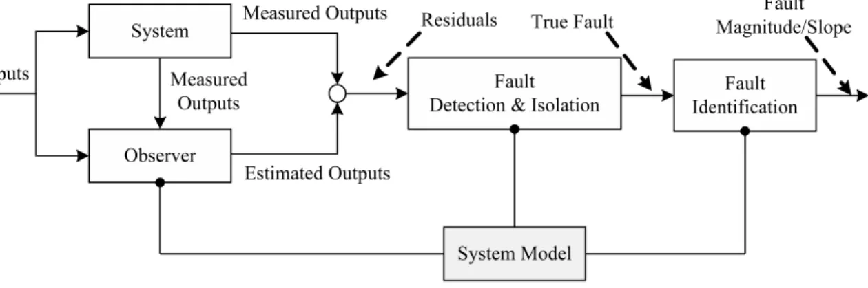
Fig. 2 shows the architecture of a generic model-based diagnosis approach. In this scheme, the model is used to represent the expected behavior of a system under nominal and faulty conditions. A mathematical model capturing the relation between the input signals and the output measurements is used to track or estimate the system outputs based on the observed measurements. The resulting dierences between estimated and measured outputs, or residuals, are processed to detect, isolate, and identify the true fault(s). With a perfect model, and no measurement noise, a zero residual implies nominal operating conditions, while a non-zero residual implies the presence of faults. In practical applications, however, a residual is seldom zero under nominal operating conditions due to the presence of noise in the measurements and imperfections in the models employed. Hence, statistical mechanisms have been developed to mitigate the eects of modeling abstractions and measurement noise. These statistical methods increase the robustness of model-based detection and isolation approaches and reduce the generation of false alarms [26]. While early detection and isolation of faults is imperative in safety-critical systems, fault identication is important for fault- adaptive control [27] and prognosis [28]. The fault detection and isolation steps can be aggregated into one decision making scheme (e.g., see [26,29]), or solved as sequential problems (e.g., [7]), where the fault isolation module is invoked once the fault detection mechanism indicates the occurrence of a fault. Once the true fault is isolated, the magnitude or slope of this fault is estimated through fault identication.

Based on the reasoning strategy employed, model-based approaches can be broadly classied as abductive and consistency-based. Abductive approaches reason from eects to causes, while consistency-based approaches reason from causes to eect. In abductive approaches, the observed measurements are compared to the expected nominal behavior of the system, and any discrepancy between the two is explained by the diagnosis, which is dened as a set of abnormality assumptions

(23)

Figure 2: The architecture of a generic model-based diagnosis approach.

that covers (or, in terms of logic, implies) the observations [30]. On the other hand, in consistency- based diagnosis approaches, diagnosis involves identifying the minimal set of faulty components, which along with the assumption that all other components are not faulty, makes the system model consistent with the observed sensor measurements [21,30,31].

Dynamic physical processes are, in reality, continuous-time processes, where the system behavior is dened at every instance of dense time. However, all automated diagnostic tools implemented on computers use sampled data. Hence, to facilitate the simulation and analysis of these models using digital computers, discrete-time models are developed where the system behavior is dened at discrete time points. In our work, we will focus on discrete-time models of dynamic systems. At the highest level of abstraction, a dynamic system can be represented as discrete-event-system (DES) representations, where time is not explicit in the system behavior. Instead, system behavior is dened by transitions between pre-dened symbolic states, and these transitions are governed by pre-dened events. At a lower level of abstraction, the system behavior can be represented using qualitative models, wherein the relationships between faults and symptoms, as well as evolution of system dynamics, are represented by qualitative expressions. At the next level of abstraction, the system behavior is dened using state-space, or input-output equations [2]. The diagnosis approaches that use the above mentioned models must be eective in diagnosing faults in real-world scenarios, where uncertainties created by sensor noise and modeling abstractions cannot be avoided. Uncertainty present in noise sensor readings, and inaccurate system models are captured by probabilistic and fuzzy-set driven schemes [32], or by interval methods [33]. In our research, we use the probabilistic framework for uncertainty, and review reasoning schemes based on Bayesian methods for robust diagnosis [3,34]. Hence, at the lowest level of abstraction, we use models of dynamic systems which explicitly capture these uncertainties. Example of such models include Bayesian networks, hidden Markov models, and Dynamic Bayesian networks [3].

(24)

Robust Model-Based Fault Diagnosis Approaches

Uncertainties are unavoidable in the real world. There are several possible causes of uncertainty, such as modeling inaccuracies that can be attributed to modeling abstractions and parameter uncertainties, sensor noise, disturbances, and process noise. These topics are discussed in greater detail below:

1. Modeling inaccuracies: The main causes of modeling inaccuracies are (i) modeling abstractions, and (ii) parametric uncertainties. Models rarely capture the exact dynamics of a real system, mainly because it is seldom possible to know everything about a system. Further- more, modeling complex nonlinearities present in the system in a suciently precise form is dicult. Hence, a system model is usually an abstraction of the actual system behavior. For example, complex nonlinear models are simplied by linearizing the parameters, or reducing the order of the nonlinearity. During abstraction or simplication, the modeler focuses on the important behaviors of the system while avoiding computational intractability, and reducing the modeling eort that would be required to capture every small detail of system behavior.

As a result, the predicted model behaviors will invariably have certain dierences from the actual underlying system behavior. Moreover, building a complete system model requires detailed knowledge of the system conguration and component behaviors, as well as component parameters. This knowledge is typically obtained by consulting system designers and experts, extracting information from device manuals and research papers, and using experimental data collected during system operations. When experimental data is used, unknown parameters and function relations associated with the models are estimated using system identication techniques. Methods for estimation of system parameters are seldom exact, and estimated parameter values and their functional forms are generally approximations of the actual parameter values. Inaccurate parameter estimates also result in uncertainties in system behavior.

Modeling errors usually have a multiplicative eect on the system behavior.

2. Sensor noise: Most real world sensors are noisy, and the noise may or may not conform to known probability distributions. However, for practical purposes, noise is typically modeled as a random Gaussian white noise with known parametric or non-parametric stochastic distributions.

3. Disturbances and Process noise: Disturbances are usually modeled as unknown extra inputs acting on the plant. For the purpose of fault diagnosis, disturbances are considered

(25)

as nuisance variables, the presence of which the diagnosis approach must ignore and be unaected by. Process noise captures the dierence between the actual observed evolution of state variables based on the values of the states in the previous time step as compared to the state evolution modeled by our system models.

Other causes of uncertainty may also be present. For example, in large systems, information is often carried to dierent parts of the system, as well as, to the reasoners, via information networks which introduce additional uncertainty, because the transmission may result in dropping of information packets and transposing of observation sequences. However, modeling these forms of uncertainty is beyond the scope of this dissertation.

1. Robustness through modeling abstractions: Dierent model-based diagnosis schemes handle these uncertainties in dierent ways. Discrete-event systems [5, 35, 36] and the qualitative simulation-based diagnosis schemes [3740] address the uncertainties through modeling abstractions. The DES schemes abstract the system dynamics into a set of discrete modes and events, while the qualitative model-based diagnosis schemes abstract the system evolution in terms of qualitative dierential equations and abstracted qualitative behaviors.

2. Handling disturbances through decoupling: The analytical redundancy relation-based approaches [2] handle uncertainties modeled as additive disturbances by decoupling their eect on the outputs through algebraic matrix manipulation.

3. Handling parameter uncertainties by accommodating parameter variations: An- other approach to handle uncertainty is presented in [41], where the system parameters are modeled as intervals, rather than constants, and sensitivity analysis of the generated residuals is used to correctly evaluate the fault residuals for diagnosis.

4. Handling process and sensor noise through probabilistic approaches: Probabilistic model-based diagnosis schemes handle sensor and process noise within the same framework using probability theory that provides a mathematically sound reasoning mechanism for diagnosis under uncertainty. These approaches uses probabilistic models, such as Bayesian networks and Dynamic Bayesian networks [3] to explicitly model measurement noise and modeling inaccuracies, and use Bayesian reasoning techniques to generate correct diagnosis results in the presence of uncertainties.

In the remainder of this chapter, we present and compare the dierent model-based diagnosis

(26)

that use discrete-event system models, followed by qualitative diagnosis of dynamic systems. Then we present analytical redundancy-based diagnosis schemes, followed by probabilistic model-based diagnosis schemes.

Discrete-Event Systems Diagnosis

Wonham, in [42], denes a discrete event system (DES) representation of a dynamic system to be equipped with a state space and state-transition structure. In particular, a DES is discrete in time and (usually) in state space; it is asynchronous or event-driven: that is, driven by events other than, or in addition to, the tick of a clock. Finite state machines (FSMs) have been widely used for modeling DES [43]. FSMs are graphs where nodes represent states, and edges represent transitions that can be taken from one state to another if the event guarding the transition occurs [43]. Formally FSMs can be represented as a tuple(Σ, S, S0, δ, F), whereΣis the input alphabet,S is a nite non empty set of states,S0⊆S is the set of initial states,δ:S×Σ→S is the state transition function, and F ⊆S is the set of nal states. FSMs allow for intuitive modeling of systems and match the mental models many people use to analyze complex systems [36]. Also, capturing the ordering of events is straightforward using FSMs. However, as we will show in the remainder of this section, generation of FSMs usually involves quantization of the continuous, and depending on how ne this quantization is, FSMs can suer from high space complexity, and result in the FSM-based DES diagnosis schemes to be computationally very expensive [5,35, 36].

Example. Consider the two-tank example shown in Fig. 3. The uid level in the tanks represent the system state. A discrete, quantized state space representation for the tank system involves representing the liquid levels into High, Medium, Low, and Empty, as shown in the gure. Here, the state of the two tank system can be dened as an ordered pair(s_tank₁, s_tank₂), wheres_tank₁ is the quantized state of tank1ands_tank₂is the quantized state of tank2. In total, there are sixteen states possible quantized states in the two tank system, as shown in Fig. 4, with state1 corresponding to both tanks being Empty, i.e.,(Empty, Empty), state2 corresponding to the(Low, Empty)state for two tanks, and so on. One possible FSM for the two tank system is shown in Fig. 5. Assume the uid inowFinto be constant. Under normal operation, the system starts in(Empty, Empty). Then as water ows into tank1, the system moves to(Low, Empty)and stays in this state till the water level in tank 1 reaches pipe R12. After this, the state changes to(M edium, Empty), water starts to ow into tank 2, and the system-state changes to (M edium, Low). Then, the system moves into(M edium, M edium), and nally to(High, High). The states mentioned above are the

(27)

Figure 3: Schematic of a two tank system with quantized states.

Figure 4: Quantized state-space of the two-tank system. Grey arrows depict normal transitions, the black arrow shows an unobservable faulty transition.

nominal states. States other than these can be considered faulty states and can be reached through transitions caused by faults, such as the transition from(M edium, M edium)to(High, M edium) (shown by a black arrow in Fig. 4) could be a result of an abrupt blockage in pipeR12. Similarly, a leak in pipeR1 could result in the system going to(Low, M edium)from(M edium, M edium). In the DES framework, faults are usually modeled as unobservable transition events.

The diagnosis approaches available in literature for discrete event approaches can be classied as one of two types: event-based and state-based [36]. In event-based diagnosis approaches, faults are modeled as unobservable events, otherwise, they are trivially diagnosable. Fault diagnosis in event- based frameworks typically involves inference to be made about the occurrence of unobservable failure events based on observed events. In state-based approaches, the state-space is partitioned according to the failure status of the system, into nominal and faulty modes, and the problem of fault diagnosis involves the determination of whether the system is in nominal or faulty mode based on the most recent observed measurements.

(28)

Figure 5: A FSM for the two-tank system.

An event-based DES diagnosis framework is presented in [5, 44]. The system is modeled as a FSM, and has both observable and unobservable events. Observable events can include controller commands and sensor readings. Unobservable events consist of fault events and other events which cause state transitions that are not observable by the sensors. At the core of this diagnostic method- ology is a diagnoser that is modeled as a deterministic FSM and systematically generated oine from the system model. This diagnoser serves as an extended observer, and gives estimates of the current state of the system after the occurrence of every observable event. The transitions of diagnoser FSM are only based on observable events. The state of a diagnoser consists of estimated current system states, and a failure label which indicates whether a faulty transition of that specic type necessarily had to be taken for the system to reach the estimated state. A fault is unequivocally diagnosed when a state in the diagnoser is reached, wherein each system state estimate has the fault label corresponding to this fault.

A state-based DES diagnosis scheme is described in [36], where the system is modeled as a Moore FSM, so that each state of the system represents a system condition (or, failure mode). Being state- based, the goal of this diagnosis scheme is to identify the failure mode the system is in, rather than explicit failure events that caused the system to be in this mode, as is the case for event-based DES diagnosis schemes. State-based diagnosis schemes are useful because for most practical settings, system models are constructed by composing several smaller component models, each usually having a single nominal mode and a few failure modes. Hence, a direct relation exists between system state and the failure mode. This approach assumes that a system has a single nominal mode and several failure modes. Like [5,44], this approach also generates a diagnoser, which takes as input the output sequence of the system and estimates the failure mode of the system. The states in the diagnoser contain an output, possible system states consistent with the output sequence, and possible system condition estimate associated with these states. If in a diagnoser state, an output is possible from

(29)

its set of system states, a transition is created from this diagnoser state to the next diagnoser state corresponding to that output, and the new system states that could have been reached from the possible system states. The possible system conditions for this new state is also marked accordingly.

A fault state is diagnosed when it is estimated with certainty that the system is in that particular fault state.

The diagnosability property of DES-based schemes is studied in [5, 44] and [36]. A fault event or mode is considered to be diagnosable if it can be detected and isolated after the occurrence of a nite number of events following the failure event. In addition, [5, 44] also dene the notion of I-Diagnosability. A system is I-Diagnosable if it can be detected and isolated within a nite number of events following the occurrence of an indicator event corresponding to that fault.

Even though there are similarities between the approaches presented in [5] and [36], there are some inherent dierences between the two approaches. In [36], the authors assume that the states of the system can be partitioned according to the condition (failure mode) of the system. Therefore, their focus is on determining the system condition rather than detecting failure events. This approach, therefore, allows diagnosis of faults in situations where the fault event has occurred before the start of diagnosis. Moreover, the assumption simplies the transition function of the state-based diagnoser in [36] because the system condition is assumed to be a function of the system state, and avoids the need for propagating fault labels, as is done in the event-based diagnoser in [5,44].

Another state-based, consistency-based DES diagnosis scheme is presented in [35], wherein the continuous state-space is partitioned and the system is represented as a timed discrete-event model.

A quantizer partitions the quantitative state-space of the system into a nite set of qualitatively similar states, each represented by a qualitative value. The quantizer also generates an event every time the system moves from one quantized state to another. The diagnosis approach uses the timed event sequences, along with timed input sequences, to diagnose the system. Quantization results in nondeterminism in the model, since for a known quantized state and known input, it may be possible for the system to enter more than one new quantized state, as the exact point in the quantized space is not known. To represent the non-determinism in its behavior, the author models the system as a semi-Markov process in a compact manner. Based on the sequence of inputs and possible events, the diagnoser computes the probabilities of faults, and as more events occur, the probability of the true fault will increase in value, while for other faults, the probability should eventually become negligible. If at the end of diagnosis, no fault can be uniquely diagnosed, the relative ranking of the probabilities gives an indication of the likelihood of dierent fault hypotheses.

(30)

Discussion

DES models handle robustness to uncertainties by abstracting away details from continuous systems, and representing the system dynamics in terms of discrete states and events. Once abstracted, the DES diagnosis schemes can be applied to these DES models without additional mechanisms for handling uncertainty. Note, however, that decisions about whether the system is in a particular state or where a particular event has occurred must still be taken in the presence of uncertainties in system dynamics at the lowest level of abstraction. As a result, the task of handling such uncertainties is delegated to these decision tasks, so that once it is determined, taking into account uncertainties, that a system is in a particular state and a certain event has occurred, the DES diagnosis approaches can generate correct diagnosis results in the presence of uncertainties without explicitly having to handle such uncertainties.

The abstraction of details in a DES has a trade-o. If the level of abstraction is very high compared to the actual system behavior, information crucial to fast and accurate diagnosis of faults is lost. A detailed DES model at a lower level of abstraction can overcome this drawback, but would increase the size of the model and the computation time for the DES diagnosis schemes.

Moreover, the model may be dicult to develop. Generation of DES models require quantization of the continuous system state-space. Quantization can be leveraged to build both untimed and timed models. Timed DES models capture information about system dynamics beyond that obtained from a simple ordering of events. Quantization seems to be appropriate for systems with discrete inputs, sensors and discrete faults. If the sensors are not discrete, quantization loses information.

Moreover, quantization based approaches suer from state explosion depending on the resolution of quantization of its state-space. In addition, to use these approaches, faults have to be quantized as well. Also, if the faults are possible in any state of the system, then the DES model becomes very large. In [1], the author presents an approach for constructing a DES model for continuous systems by systematically abstracting the dynamics of the observed measurements in the presence of dierent faults to relatively avoid the exponential blow-up of states and state-transitions. The DES diagnosis schemes provide a well-developed framework for event-based and state-based fault diagnosis. But, they lack sophisticated mechanisms to handle measurement noise and unknown disturbances that cannot be avoided in practical scenarios. In addition, the performance of DES diagnosis schemes depend on the order in which the input and output events are observed, and if the order in which events are generated by the system is not the same as that observed by the diagnoser, or if some

(31)

observed events are missing, the DES diagnosis approaches may fail to generate correct diagnosis results.

Diagnosis Using Qualitative Models

Qualitative models express the relationships between observed symptoms and the faults, as well as the system dynamics in terms of qualitative functions and equations [45]. The qualitative diagnosis schemes leverage the cause-eect relation behavior for dierent faults captured in the qualitative models to correctly isolate faults. Rather than focusing on expert systems which useIF−T HEN− ELSE rules [34], we will focus our discussion on those qualitative model-based diagnosis schemes that are derived from rst-principles and a sound understanding of the physics of the system. In the following, we present a few qualitative model-based diagnosis approaches.

Several qualitative diagnosis schemes, such as [37, 38, 46, 47], use signed digraphs (SDGs) for diagnosis. An SDG is a directed graph whose nodes represent deviation from the steady state of a variable, and signed arcs represent the relationships between these nodes [38]. SDGs are much more compact than truth tables, decision tables, or nite state models.

Example. For example, if we denote the uid-level of a tank asH, its inlet ow asFin, its outlet ow asFout, and the resistance of its outlet pipe asRout, then the equations to represent this system are [45]:

F_in−F_out = dH dt Fout = H

R_out.

The corresponding SDG for this system is given in Fig. 6. An external change causing the ow rate Fin to change, would cause dH and H to change in the same direction, which will in turn cause Foutto also change similarly. However, this change in theFout would cause thedH to change in the other direction, implying a feedback. The SDG can be obtained by abstracting the mathematical model of the underlying process.

In [38], the authors derive a cause-eect (CE) graph from a system's SDG. The CE graph consists of only valid nodes (i.e., nodes which are abnormal) and consistent arcs (i.e., arcs which explain the local propagation of the fault and hence, the observed symptom). The sign of the nodes in a SDG can be considered as a pattern which may match a particular fault condition, and a fault is isolated

(32)

Figure 6: Signed digraph for a simple tank system.

known, a partial pattern is formed, and this indicates the possibility of all possible fault conditions the partial pattern corresponds to being present. In [37], the arcs gains of SDGs are allowed to vary dynamically, thereby allowing modeling of nonlinearities. In [46], the authors address the issue of conditional arcs in SDGs. SDGs can get quite complicated for complex systems, and in [47], the authors present techniques to simplify the SDGs for fault diagnosis. A rule-based approach to diagnosis using SDGs is presented in [48], where logical statements, or rules, such as,IF−(SDG rule premise)−T HEN−(possible fault), are automatically derived from SDGs and these statements are evaluated using online data to generate the diagnosis result. These automatically derived rules can also be integrated with other rules using an expert system framework, such as forward chaining [34].

A method for qualitative analysis of causal feedback in SDGs is proposed in [49] to resolve feedback ambiguities, and this method is implemented in a simulator for qualitative ordinary dierential equations, called QUAF.

A qualitative simulation (QSIM)-based diagnosis approach, Mimic, is presented in [39,40], where the system is modeled using qualitative dierential algebraic equations (QDAEs). QDAEs are a general, implicit form of qualitative dierential equations (QDEs) [50]. Given a set of ordinary dierential equations (ODEs), QDEs can be considered as an abstraction of these ODEs, and represented by a set of qualitative constraint equations which are satised by any behavior that satises the given ODEs [50]. The constraint equations consist of a set of symbols representing the process variables, and a set of constraints on how these variables may be related to each other. The constraints allow the expression of simple mathematical relationships between the variables such as addition, multiplication, and dierentiation. The evolution of the system is qualitatively simulated (see [50]), where essentially, the innite number of numeric behaviors of a system is discretized into a smaller set of qualitatively distinct behaviors or states, and qualitative transitions exist between states, depending on the constraints.

In Mimic, given the nominal model of the system, QSIM starts at the initial state, and as and when observations change, the qualitative model is simulated based on the observations, predicting the immediate successor qualitative states the system might possibly be in. In addition, QSIM also